This is a static, non-editable tutorial.
We recommend you install QuCumber if you want to run the examples locally.
You can then get an archive file containing the examples from the relevant release
here.
Alternatively, you can launch an interactive online version, though it may be a bit slow:
![]()
Reconstruction of a complex wavefunction
In this tutorial, a walkthrough of how to reconstruct a complex wavefunction via training a Restricted Boltzmann Machine (RBM), the neural network behind QuCumber, will be presented.
The wavefunction to be reconstructed
The simple wavefunction below describing two qubits (coefficients stored in qubits_psi.txt) will be reconstructed.

where the exact values of  and
and  used for this tutorial are

The example dataset, qubits_train.txt, comprises of 500  measurements made in various bases (X, Y and Z). A corresponding file containing the bases for each data point in
 qubits_train.txt, qubits_train_bases.txt, is also required. As per convention, spins are represented in binary notation with zero and one denoting spin-down and spin-up, respectively.
Using qucumber to reconstruct the wavefunction
Imports
To begin the tutorial, first import the required Python packages.
[1]:
import numpy as np
import torch
import matplotlib.pyplot as plt

from qucumber.nn_states import ComplexWaveFunction

from qucumber.callbacks import MetricEvaluator

import qucumber.utils.unitaries as unitaries
import qucumber.utils.cplx as cplx

import qucumber.utils.training_statistics as ts
import qucumber.utils.data as data
import qucumber

# set random seed on cpu but not gpu, since we won't use gpu for this tutorial
qucumber.set_random_seed(1234, cpu=True, gpu=False)
The Python class ComplexWaveFunction contains generic properties of a RBM meant to reconstruct a complex wavefunction, the most notable one being the gradient function required for stochastic gradient descent.
To instantiate a ComplexWaveFunction object, one needs to specify the number of visible and hidden units in the RBM. The number of visible units, num_visible, is given by the size of the physical system, i.e. the number of spins or qubits (2 in this case), while the number of hidden units, num_hidden, can be varied to change the expressiveness of the neural network.
Note: The optimal num_hidden : num_visible ratio will depend on the system. For the two-qubit wavefunction described above, good results can be achieved when this ratio is 1.
On top of needing the number of visible and hidden units, a ComplexWaveFunction object requires the user to input a dictionary containing the unitary operators (2x2) that will be used to rotate the qubits in and out of the computational basis, Z, during the training process. The unitaries utility will take care of creating this dictionary.
The MetricEvaluator class and training_statistics utility are built-in amenities that will allow the user to evaluate the training in real time.
Lastly, the cplx utility allows QuCumber to be able to handle complex numbers as they are not currently supported by PyTorch.
Training
To evaluate the training in real time, the fidelity between the true wavefunction of the system and the wavefunction that QuCumber reconstructs,  , will be calculated along with the Kullback-Leibler (KL) divergence (the RBM’s cost function). First, the training data and the true wavefunction of this system need to be loaded using the
 data utility.
[2]:
train_path = "qubits_train.txt"
train_bases_path = "qubits_train_bases.txt"
psi_path = "qubits_psi.txt"
bases_path = "qubits_bases.txt"

train_samples, true_psi, train_bases, bases = data.load_data(
    train_path, psi_path, train_bases_path, bases_path
)
The file qubits_bases.txt contains every unique basis in the qubits_train_bases.txt file. Calculation of the full KL divergence in every basis requires the user to specify each unique basis.
As previously mentioned, a ComplexWaveFunction object requires a dictionary that contains the unitary operators that will be used to rotate the qubits in and out of the computational basis, Z, during the training process. In the case of the provided dataset, the unitaries required are the well-known  , and
, and  gates. The dictionary needed can be created with the following command.
[3]:
unitary_dict = unitaries.create_dict()
# unitary_dict = unitaries.create_dict(<unitary_name>=torch.tensor([[real part],
#                                                                   [imaginary part]],
#                                                                  dtype=torch.double)
If the user wishes to add their own unitary operators from their experiment to unitary_dict, uncomment the block above. When unitaries.create_dict() is called, it will contain the identity and the and gates by default under the keys “Z”, “X” and “Y”, respectively.
The number of visible units in the RBM is equal to the number of qubits. The number of hidden units will also be taken to be the number of visible units.
[4]:
nv = train_samples.shape[-1]
nh = nv

nn_state = ComplexWaveFunction(
    num_visible=nv, num_hidden=nh, unitary_dict=unitary_dict, gpu=False
)
If gpu=True (the default), QuCumber will attempt to run on a GPU if one is available (if one is not available, QuCumber will fall back to CPU). If one wishes to guarantee that QuCumber runs on the CPU, add the flag gpu=False in the ComplexWaveFunction object instantiation.
Now the hyperparameters of the training process can be specified.
epochs: the total number of training cycles that will be performed (default = 100)pos_batch_size: the number of data points used in the positive phase of the gradient (default = 100)neg_batch_size: the number of data points used in the negative phase of the gradient (default =pos_batch_size)k: the number of contrastive divergence steps (default = 1)lr: the learning rate (default = 0.001)Note: For more information on the hyperparameters above, it is strongly encouraged that the user to read through the brief, but thorough theory document on RBMs. One does not have to specify these hyperparameters, as their default values will be used without the user overwriting them. It is recommended to keep with the default values until the user has a stronger grasp on what these hyperparameters mean. The quality and the computational efficiency of the training will highly depend on the choice of hyperparameters. As such, playing around with the hyperparameters is almost always necessary.
The two-qubit example in this tutorial should be extremely easy to train, regardless of the choice of hyperparameters. However, the hyperparameters below will be used.
[5]:
epochs = 500
pbs = 100  # pos_batch_size
nbs = pbs  # neg_batch_size
lr = 0.1
k = 10
For evaluating the training in real time, the MetricEvaluator will be called to calculate the training evaluators every 10 epochs. The MetricEvaluator requires the following arguments.
period: the frequency of the training evaluators being calculated (e.g.period=200means that theMetricEvaluatorwill compute the desired metrics every 200 epochs)A dictionary of functions you would like to reference to evaluate the training (arguments required for these functions are keyword arguments placed after the dictionary)
The following additional arguments are needed to calculate the fidelity and KL divergence in the training_statistics utility.
target_psi(the true wavefunction of the system)space(the entire Hilbert space of the system)
The training evaluators can be printed out via the verbose=True statement.
Although the fidelity and KL divergence are excellent training evaluators, they are not practical to calculate in most cases; the user may not have access to the target wavefunction of the system, nor may generating the Hilbert space of the system be computationally feasible. However, evaluating the training in real time is extremely convenient.
Any custom function that the user would like to use to evaluate the training can be given to the MetricEvaluator, thus avoiding having to calculate fidelity and/or KL divergence. As an example, functions that calculate the the norm of each of the reconstructed wavefunction’s coefficients are presented. Any custom function given to MetricEvaluator must take the neural-network state (in this case, the ComplexWaveFunction object) and keyword arguments. Although the given example
requires the Hilbert space to be computed, the scope of the MetricEvaluator’s ability to be able to handle any function should still be evident.
[6]:
def alpha(nn_state, space, **kwargs):
    rbm_psi = nn_state.psi(space)
    normalization = nn_state.normalization(space).sqrt_()
    alpha_ = cplx.norm(
        torch.tensor([rbm_psi[0][0], rbm_psi[1][0]], device=nn_state.device)
        / normalization
    )

    return alpha_


def beta(nn_state, space, **kwargs):
    rbm_psi = nn_state.psi(space)
    normalization = nn_state.normalization(space).sqrt_()
    beta_ = cplx.norm(
        torch.tensor([rbm_psi[0][1], rbm_psi[1][1]], device=nn_state.device)
        / normalization
    )

    return beta_


def gamma(nn_state, space, **kwargs):
    rbm_psi = nn_state.psi(space)
    normalization = nn_state.normalization(space).sqrt_()
    gamma_ = cplx.norm(
        torch.tensor([rbm_psi[0][2], rbm_psi[1][2]], device=nn_state.device)
        / normalization
    )

    return gamma_


def delta(nn_state, space, **kwargs):
    rbm_psi = nn_state.psi(space)
    normalization = nn_state.normalization(space).sqrt_()
    delta_ = cplx.norm(
        torch.tensor([rbm_psi[0][3], rbm_psi[1][3]], device=nn_state.device)
        / normalization
    )

    return delta_
Now the basis of the Hilbert space of the system must be generated in order to compute the fidelity, KL divergence, and the dictionary of functions the user would like to compute. These metrics will be evaluated every period epochs, which is a parameter that must be given to the MetricEvaluator.
Note that some of the coefficients are not being evaluated as they are commented out. This is simply to avoid cluttering the output, and may be uncommented by the user.
[7]:
period = 25
space = nn_state.generate_hilbert_space()

callbacks = [
    MetricEvaluator(
        period,
        {
            "Fidelity": ts.fidelity,
            "KL": ts.KL,
            "normα": alpha,
            # "normβ": beta,
            # "normγ": gamma,
            # "normδ": delta,
        },
        target=true_psi,
        bases=bases,
        verbose=True,
        space=space,
    )
]
Now the training can begin. The ComplexWaveFunction object has a function called fit which takes care of this.
[8]:
nn_state.fit(
    train_samples,
    epochs=epochs,
    pos_batch_size=pbs,
    neg_batch_size=nbs,
    lr=lr,
    k=k,
    input_bases=train_bases,
    callbacks=callbacks,
    time=True,
)
Epoch: 25       Fidelity = 0.940240     KL = 0.032256   normα = 0.258429
Epoch: 50       Fidelity = 0.974944     KL = 0.017143   normα = 0.260490
Epoch: 75       Fidelity = 0.984727     KL = 0.012232   normα = 0.270684
Epoch: 100      Fidelity = 0.987769     KL = 0.010389   normα = 0.269163
Epoch: 125      Fidelity = 0.988929     KL = 0.009581   normα = 0.261813
Epoch: 150      Fidelity = 0.989075     KL = 0.009273   normα = 0.271764
Epoch: 175      Fidelity = 0.989197     KL = 0.008928   normα = 0.267943
Epoch: 200      Fidelity = 0.989451     KL = 0.008817   normα = 0.259327
Epoch: 225      Fidelity = 0.990894     KL = 0.007215   normα = 0.269941
Epoch: 250      Fidelity = 0.991517     KL = 0.006804   normα = 0.261673
Epoch: 275      Fidelity = 0.991808     KL = 0.006408   normα = 0.261002
Epoch: 300      Fidelity = 0.992318     KL = 0.005788   normα = 0.274654
Epoch: 325      Fidelity = 0.992078     KL = 0.005881   normα = 0.266831
Epoch: 350      Fidelity = 0.991938     KL = 0.006020   normα = 0.262980
Epoch: 375      Fidelity = 0.991670     KL = 0.006181   normα = 0.270877
Epoch: 400      Fidelity = 0.992082     KL = 0.005945   normα = 0.255576
Epoch: 425      Fidelity = 0.992678     KL = 0.005130   normα = 0.259746
Epoch: 450      Fidelity = 0.993102     KL = 0.004702   normα = 0.259373
Epoch: 475      Fidelity = 0.993109     KL = 0.004765   normα = 0.255803
Epoch: 500      Fidelity = 0.992805     KL = 0.004785   normα = 0.261486
Total time elapsed during training: 49.059 s
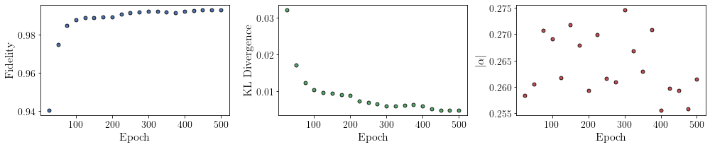
All of these training evaluators can be accessed after the training has completed, as well. The code below shows this, along with plots of each training evaluator versus the training cycle number (epoch).
[9]:
# Note that the key given to the *MetricEvaluator* must be
# what comes after callbacks[0].
fidelities = callbacks[0].Fidelity

# Alternatively, we may use the usual dictionary/list subscripting
# syntax. This is useful in cases where the name of the metric
# may contain special characters or spaces.
KLs = callbacks[0]["KL"]
coeffs = callbacks[0]["normα"]
epoch = np.arange(period, epochs + 1, period)
[10]:
# Some parameters to make the plots look nice
params = {
    "text.usetex": True,
    "font.family": "serif",
    "legend.fontsize": 14,
    "figure.figsize": (10, 3),
    "axes.labelsize": 16,
    "xtick.labelsize": 14,
    "ytick.labelsize": 14,
    "lines.linewidth": 2,
    "lines.markeredgewidth": 0.8,
    "lines.markersize": 5,
    "lines.marker": "o",
    "patch.edgecolor": "black",
}
plt.rcParams.update(params)
plt.style.use("seaborn-deep")
[11]:
fig, axs = plt.subplots(nrows=1, ncols=3, figsize=(14, 3))
ax = axs[0]
ax.plot(epoch, fidelities, "o", color="C0", markeredgecolor="black")
ax.set_ylabel(r"Fidelity")
ax.set_xlabel(r"Epoch")

ax = axs[1]
ax.plot(epoch, KLs, "o", color="C1", markeredgecolor="black")
ax.set_ylabel(r"KL Divergence")
ax.set_xlabel(r"Epoch")

ax = axs[2]
ax.plot(epoch, coeffs, "o", color="C2", markeredgecolor="black")
ax.set_ylabel(r"$\vert\alpha\vert$")
ax.set_xlabel(r"Epoch")

plt.tight_layout()
plt.show()
It should be noted that one could have just run nn_state.fit(train_samples) using the default hyperparameters and no training evaluators, which would induce different convergence behavior.
At the end of the training process, the network parameters (the weights, visible biases, and hidden biases) are stored in the ComplexWaveFunction object. One can save them to a pickle file, which will be called saved_params.pt, with the following command.
[12]:
nn_state.save("saved_params.pt")
This saves the weights, visible biases and hidden biases as torch tensors under the following keys: weights, visible_bias, hidden_bias.