This is a static, non-editable tutorial.

We recommend you install QuCumber if you want to run the examples locally. You can then get an archive file containing the examples from the relevant release here. Alternatively, you can launch an interactive online version, though it may be a bit slow:

Sampling and calculating observables

Generate new samples

Firstly, to generate meaningful data, an RBM needs to be trained. Please refer to the tutorials 1 and 2 on training an RBM-based Neural-Network-State if doing so using QuCumber is unclear. A Neural-Network-State (nn_state) of a positive-real wavefunction describing a transverse-field Ising model (TFIM) with 10 sites has already been trained in the first tutorial, with the parameters of the machine saved here as saved_params.pt. The autoload function can be employed here to instantiate the corresponding PositiveWaveFunction object from the saved nn_state parameters.

import numpy as np
import torch
import matplotlib.pyplot as plt

import qucumber
from qucumber.nn_states import PositiveWaveFunction, DensityMatrix
from qucumber.observables import ObservableBase
from qucumber.observables.pauli import flip_spin
from qucumber.utils import cplx

from quantum_ising_chain import TFIMChainEnergy, Convergence

# set random seed on cpu but not gpu, since we won't use gpu for this tutorial
qucumber.set_random_seed(1234, cpu=True, gpu=False)
nn_state = PositiveWaveFunction.autoload("saved_params.pt", gpu=False)

A PositiveWaveFunction object has a property called sample that allows us to sample the learned distribution of TFIM chains. The it takes the following arguments (along with a few others which are not relevant for our purposes):

1. k: the number of Gibbs steps to perform to generate the new samples. Increasing this number will produce samples closer to the learned distribution, but will require more computation.

2. num_samples: the number of new data points to be generated

new_samples = nn_state.sample(k=100, num_samples=10000)
print(new_samples)

tensor([[1., 0., 1.,  ..., 1., 1., 1.],
        [0., 0., 0.,  ..., 0., 0., 1.],
        [0., 0., 0.,  ..., 1., 0., 1.],
        ...,
        [0., 0., 0.,  ..., 0., 1., 1.],
        [0., 0., 0.,  ..., 0., 0., 0.],
        [0., 1., 1.,  ..., 0., 0., 0.]], dtype=torch.float64)

Magnetization

With the newly generated samples, the user can now easily calculate observables that do not require any information associated with the wavefunction and hence the nn_state. These are observables which are diagonal in the computational (Pauli Z) basis. A great example of this is the magnetization (in the Z direction). To calculate the magnetization, the newly-generated samples must be converted to 1 from 1 and 0, respectively. The function below does the trick.

def to_pm1(samples):
    return samples.mul(2.0).sub(1.0)

Now, the (absolute) magnetization in the Z-direction is calculated as follows.

def Magnetization(samples):
    return to_pm1(samples).mean(1).abs().mean()


magnetization = Magnetization(new_samples).item()

print("Magnetization = %.5f" % magnetization)

Magnetization = 0.55752

The exact value for the magnetization is 0.5610.

The magnetization and the newly-generated samples can also be saved to a pickle file along with the nn_state parameters in the PositiveWaveFunction object.

nn_state.save(
    "saved_params_and_new_data.pt",
    metadata={"samples": new_samples, "magnetization": magnetization},
)

The metadata argument in the save function takes in a dictionary of data that you would like to save alongside the nn_state parameters.

Calculate an observable using the Observable module

Magnetization (again)

QuCumber provides the Observable module to simplify estimation of expectations and variances of observables in memory efficient ways. To start off, we’ll repeat the above example using the SigmaZ Observable module provided with QuCumber.

from qucumber.observables import SigmaZ

We’ll compute the absolute magnetization again, for the sake of comparison with the previous example. We want to use the samples drawn earlier to perform this estimate, so we use the statistics_from_samples function:

sz = SigmaZ(absolute=True)
sz.statistics_from_samples(nn_state, new_samples)

{'mean': 0.5575200000000005,
 'variance': 0.09791724132414,
 'std_error': 0.0031291730748576373,
 'num_samples': 10000}

With this function we get the variance and standard error for free. Now you may be asking: “That’s not too difficult, I could have computed those myself!”. The power of the Observable module comes from the fact that it simplifies estimation of these values over a large number of samples. The statistics function computes these statistics by generating the samples internally. Let’s see it in action:

%time sz.statistics(nn_state, num_samples=10000, burn_in=100)
# just think of burn_in as being equivalent to k for now

CPU times: user 1.74 s, sys: 0 ns, total: 1.74 s
Wall time: 504 ms

{'mean': 0.5534800000000003,
 'variance': 0.09726161576157935,
 'std_error': 0.0031186794603097535,
 'num_samples': 10000}

Let’s consider what is taking place under the hood at the moment. The statistics function is drawing 10000 samples from the given nn_state, and cycling it through the visible and hidden layers for 100 Block Gibbs steps before computing the statistics. This means that, at any given time it has to hold a matrix with 10000 rows and 10 (the number of lattice sites) columns in memory, which becomes infeasible for large lattices or if we want to use more samples to bring our standard error down. To bypass this issue, the statistics function allows us to specify the number of Markov Chains to evolve using the nn_state, and will sample from these chains multiple times to produce enough samples. It takes the following arguments:

• num_samples: the number of samples to generate internally

• num_chains: the number of Markov chains to run in parallel (default = 0, meaning num_chains = num_samples)

• burn_in: the number of Gibbs steps to perform before recording any samples (default = 1000)

• steps: the number of Gibbs steps to perform between each sample; increase this to reduce the autocorrelation between samples (default = 1)

• initial_state: the initial state of the Markov Chain. If given, num_chains will be ignored. (default = None)

• overwrite: Whether to overwrite the initial_state tensor, with the updated state of the Markov chain. (default = False)

The statistics function will also return a dictionary containing the mean, standard error (of the mean), the variance, and the total number of samples that were drawn with the keys mean, std_error, variance, and num_samples respectively.

%time sz.statistics(nn_state, num_samples=10000, num_chains=1000, burn_in=100, steps=2)

CPU times: user 331 ms, sys: 0 ns, total: 331 ms
Wall time: 83.8 ms

{'mean': 0.55116,
 'variance': 0.09716837123712346,
 'std_error': 0.003117184165831776,
 'num_samples': 10000}

Recall that, earlier, we had produced a batch of samples new_samples which we assumed were already converged to the equilibrium after 100 Gibbs steps. We can use these pre-computed samples to skip the “burn-in” phase like so:

%%time
sz.statistics(
    nn_state, num_samples=10000, burn_in=0, steps=2, initial_state=new_samples[:1000, :]
)

CPU times: user 73.9 ms, sys: 0 ns, total: 73.9 ms
Wall time: 21.6 ms

{'mean': 0.5508999999999998,
 'variance': 0.09669885988598853,
 'std_error': 0.003109644029241748,
 'num_samples': 10000}

We only took the first 1000 samples from new_samples in order to keep the number of Markov Chains the same as the previous cell. Notice how much time was saved by initializing the chains using pre-equilibrated samples. In fact, one could save even more time by skipping the generation of pre-equilibrated samples and using the nn_state’s training data instead!

In addition to using less memory (since the matrix held in memory is now of size num_chains x num_sites = 1000 x 10), using fewer chains also produced a decent speed boost! Next, we’ll try increasing the total number of drawn samples:

sz.statistics(nn_state, num_samples=int(1e7), num_chains=1000, burn_in=100, steps=2)

{'mean': 0.5505633800000023,
 'variance': 0.09801013840398955,
 'std_error': 9.900006990098014e-05,
 'num_samples': 10000000}

Note how much we reduced our standard error just by increasing the number of drawn samples. Finally, we can also draw samples of measurements of the observable using the sample function:

sz.sample(nn_state, k=100, num_samples=50)

tensor([0.2000, 1.0000, 0.0000, 0.4000, 0.2000, 0.4000, 0.4000, 0.4000, 0.6000,
        1.0000, 1.0000, 0.6000, 0.4000, 0.0000, 0.4000, 0.4000, 0.8000, 1.0000,
        0.0000, 0.4000, 0.0000, 0.0000, 0.8000, 0.8000, 0.8000, 0.8000, 0.6000,
        0.8000, 0.6000, 1.0000, 0.4000, 0.4000, 0.4000, 0.4000, 0.8000, 0.2000,
        0.2000, 0.0000, 0.8000, 0.4000, 0.6000, 0.0000, 0.2000, 1.0000, 0.4000,
        0.8000, 0.2000, 0.4000, 1.0000, 0.6000], dtype=torch.float64)

Note that this function does not perform any fancy sampling tricks like statistics and is therefore susceptible to “Out of Memory” errors.

TFIM Energy

Some observables cannot be computed directly from samples, but instead depend on the nn_state as previously mentioned. For example, the magnetization of the TFIM simply depends on the samples the user gives as input. While we did provide the nn_state as an argument when calling statistics_from_samples, SigmaZ ignores it. The TFIM energy, on the other hand, is much more complicated. Consider the TFIM Hamiltonian:

As our nn_state was trained in the Z-basis, the off-diagonal transverse-field term is impossible to compute just from the samples; we need to know the value of the wavefunction for each sample as well. An example for the computation of the energy is provided in the python file quantum_ising_chain.py, which takes advantage of QuCumber’s Observable module.

quantum_ising_chain.py comprises of a class that computes the energy of a TFIM (TFIMChainEnergy) that inherits properties from the Observable module. To instantiate a TFIMChainEnergy object, the value must be specified. The trained nn_state parameters are from the first tutorial, where the example data was from the TFIM with 10 sites at its critical point ().

h = 1

tfim_energy = TFIMChainEnergy(h)

To go ahead and calculate the mean energy and its standard error from the previously generated samples from this tutorial (new_samples), the statistics_from_samples function in the Observable module is called upon.

energy_stats = tfim_energy.statistics_from_samples(nn_state, new_samples)
print("Mean: %.4f" % energy_stats["mean"], "+/- %.4f" % energy_stats["std_error"])
print("Variance: %.4f" % energy_stats["variance"])

Mean: -1.2353 +/- 0.0005
Variance: 0.0022

The exact value for the energy is -1.2381.

To illustrate how quickly the energy converges as a function of the sampling step (i.e. the number of Gibbs steps to perform to generate a new batch of samples), steps, the Convergence function in quantum_ising_chain.py will do the trick. Convergence creates a batch of random samples initially, which is then used to generate a new batch of samples from the nn_state. The TFIM energy will be calculated at every Gibbs step. Note that this function is not available in the QuCumber API; it is only used here as an illustrative example.

steps = 200
num_samples = 10000

dict_observables = Convergence(nn_state, tfim_energy, num_samples, steps)

energy = dict_observables["energies"]
err_energy = dict_observables["error"]

step = np.arange(steps + 1)

E0 = -1.2381

ax = plt.axes()
ax.plot(step, abs((E0 - energy) / E0) * 100, color="red")
ax.hlines(abs((E0 - energy_stats["mean"]) / E0) * 100, 0, 200, color="black")
ax.set_xlim(0, steps)
ax.set_ylim(0, 0.6)
ax.set_xlabel("Gibbs Step")
ax.set_ylabel("% Error in Energy")

Text(0, 0.5, '% Error in Energy')

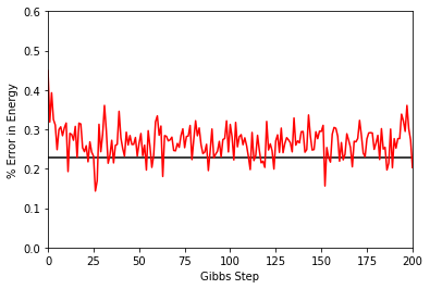
One can see a brief transient period in the magnetization observable, before the state of the machine “warms up” to equilibrium (this explains the burn_in argument we saw earlier). After that, the values fluctuate around the estimated mean (the horizontal black line).

Combining observables

One may also add / subtract and multiply observables with each other or with real numbers. To illustrate this, we will build an alternative implementation of the TFIM energy observable. First, we will introduce the built-in NeighbourInteraction observable:

from qucumber.observables import NeighbourInteraction

The TFIM chain we trained the nn_state on did not have periodic boundary conditions, so periodic_bcs=False. Meanwhile, c specifies the distance between interacting spins, that is, a given site will only interact with a site c places away from itself; we set this to 1 as the TFIM chain has nearest-neighbour interactions.

nn_inter = NeighbourInteraction(periodic_bcs=False, c=1)

Next, we need the SigmaX observable, which computes the magnetization in the X-direction:

from qucumber.observables import SigmaX

Next, we build the Hamiltonian, setting :

h = J = 1
sx = SigmaX()
tfim = -J * nn_inter - h * sx

The same statistics of this new TFIM observable can also be calculated.

new_tfim_stats = tfim.statistics_from_samples(nn_state, new_samples)
print("Mean: %.4f" % new_tfim_stats["mean"], "+/- %.4f" % new_tfim_stats["std_error"])
print("Variance: %.4f" % new_tfim_stats["variance"])

Mean: -1.2353 +/- 0.0005
Variance: 0.0022

The statistics above match with those computed earlier.

Rényi Entropy and the Swap operator

We can estimate the second Rényi Entropy using the Swap operator as shown by Hastings et al. (2010). The second Rényi Entropy, in terms of the expectation of the Swap operator is given by:

where is the subset of the lattice for which we wish to compute the Rényi entropy.

from qucumber.observables import SWAP

As an example, we will take the region consist of sites through (inclusive).

A = [0, 1, 2, 3, 4]
swap = SWAP(A)

swap_stats = swap.statistics_from_samples(nn_state, new_samples)
print("Mean: %.4f" % swap_stats["mean"], "+/- %.4f" % swap_stats["std_error"])
print("Variance: %.4f" % swap_stats["variance"])

Mean: 0.7838 +/- 0.0061
Variance: 0.3663

The second Rényi Entropy can be computed directly from the sample mean. The standard error of the entropy, from first-order error analysis, is given by the standard error of the Swap operator divided by the mean of the Swap operator.

S_2 = -np.log(swap_stats["mean"])
S_2_error = abs(swap_stats["std_error"] / swap_stats["mean"])


print("S_2: %.4f" % S_2, "+/- %.4f" % S_2_error)

S_2: 0.2437 +/- 0.0077

Writing custom diagonal observables

QuCumber has a built-in module called Observable which makes it easy for the user to compute any arbitrary observable from the nn_state. To see the the Observable module in action, an example (diagonal) observable called PIQuIL, which inherits properties from the Observable module, is shown below.

The PIQuIL observable takes a measurement at a site and multiplies it by the measurement two sites away from it. There is also a parameter, , that determines the strength of each of these interactions. For example, for the dataset and with , the PIQuIL for each data point would be and , respectively.

class PIQuIL(ObservableBase):
    def __init__(self, P):
        self.name = "PIQuIL"
        self.symbol = "Q"
        self.P = P

    # Required : function that calculates the PIQuIL. Must be named "apply"
    def apply(self, nn_state, samples):
        samples = to_pm1(samples)
        interaction_ = 0.0
        for i in range(samples.shape[-1] - 2):
            interaction_ += self.P * samples[:, i] * samples[:, i + 2]

        return interaction_


P = 0.05
piquil = PIQuIL(P)

The apply function is contained in the Observable module, but is overwritten here. The apply function in Observable will compute the observable itself and must take in the nn_state and a batch of samples as arguments. Thus, any new class inheriting from Observable that the user would like to define must contain a function called apply that calculates this new observable. For more details on apply, we refer to the documentation:

Although the PIQuIL observable could technically be computed without the first argument of apply since it does not ever use the nn_state, we still include it in the list of arguments in order to conform to the interface provided in the ObservableBase class.

Since we have already generated new samples of data, the PIQuIL observable’s mean, standard error and variance on the new data can be calculated with the statistics_from_samples function in the Observable module. The user must simply provide the nn_state and the samples as arguments.

piquil_stats1 = piquil.statistics_from_samples(nn_state, new_samples)

The statistics_from_samples function returns a dictionary containing the mean, standard error and the variance with the keys “mean”, “std_error” and “variance”, respectively.

print(
    "Mean PIQuIL: %.4f" % piquil_stats1["mean"], "+/- %.4f" % piquil_stats1["std_error"]
)
print("Variance: %.4f" % piquil_stats1["variance"])

Mean PIQuIL: 0.1762 +/- 0.0016
Variance: 0.0244

Exercise: We notice that the PIQuIL observable is essentially a scaled next-nearest-neighbours interaction. (a) Construct an equivalent Observable object algebraically in a similar manner to the TFIM observable constructed above. (b) Compute the statistics of this observable on new_samples, and compare to those computed using the PIQuIL observable.

# solve the above exercise here

Writing off-diagonal observables

Now, as the PIQuIL observable was diagonal, it was fairly easy to write. Things get a bit more complicated once we consider off-diagonal observables, as we’d need to make use of information about the quantum state itself. In general, computing an observable exactly with respect to the state requires performing a trace:

where are two orthonormal bases spanning the Hilbert space. Multiplying the numerator and denominator by gives:

Hence, computing the expectation of the observable with respect to , amounts to estimating the so-called “local-estimator” with respect to the probability distribution . Setting to our computational basis states , we note that, as we are able to draw samples from in the computational basis using our nn_state, we can easily estimate the expectation of :

where denotes the set of drawn samples. Recall that the local-estimator is:

which, in the case of a pure state , reduces to:

The task of the apply function, is actually to compute the local-estimator, given a sample . Ideally, this function would take into account the structure of in order to perform this computation efficiently, and avoid iterating through every entry of the wavefunction of density matrix unnecessarily.

It should be noted that, though the Neural-Network-States provided by QuCumber do not give normalized probability estimates, this is not an issue for computing the local-estimator, as the normalization constant cancels out.

As an example, we will write a simplified version of the SigmaX observable. But first, let’s see what the statistics of the official version of SigmaX are, for the sake of later comparison:

sx.statistics_from_samples(nn_state, new_samples)

{'mean': 0.7293210861294865,
 'variance': 0.07933831206407158,
 'std_error': 0.002816705736566594,
 'num_samples': 10000}

class MySigmaX(ObservableBase):
    def __init__(self):
        self.name = "SigmaX"
        self.symbol = "X"

    def apply(self, nn_state, samples):
        samples = samples.to(device=nn_state.device)

        # vectors of shape: (2, num_samples,)
        denom = cplx.conjugate(nn_state.psi(samples))
        numer_sum = torch.zeros_like(denom)

        for i in range(samples.shape[-1]):  # sum over spin sites
            samples_ = flip_spin(i, samples.clone())  # flip the spin at site i

            # compute the numerator of the importance and add it to the running sum
            numer = cplx.conjugate(nn_state.psi(samples_))
            numer_sum.add_(numer)

        mag = cplx.elementwise_division(numer_sum, denom)

        # take real part (imaginary part should be approximately zero)
        # and divide by number of spins
        return cplx.real(mag).div_(samples.shape[-1])

MySigmaX().statistics_from_samples(nn_state, new_samples)

{'mean': 0.7293210861294865,
 'variance': 0.07933831206407158,
 'std_error': 0.002816705736566594,
 'num_samples': 10000}

We’re on the right track! The only remaining problem is generalizing this to work with mixed states. Note that in both expressions of the local-estimator, we need to compute a ratio dependent on and . The Neural-Network-States provided by QuCumber implement the functions importance_sampling_weight, importance_sampling_numerator, and importance_sampling_denominator in order to simplify writing observables for both pure and mixed states.

In simple cases, we’d only need to make use of importance_sampling_weight, however, note that, since the denominator can be factored out of the summation, it is more efficient to compute the numerator and denominator separately in order to avoid duplicating work. Let’s update our version of the X-magnetization observable to support mixed states:

class MySigmaX(ObservableBase):
    def __init__(self):
        self.name = "SigmaX"
        self.symbol = "X"

    def apply(self, nn_state, samples):
        samples = samples.to(device=nn_state.device)

        # vectors of shape: (2, num_samples,)
        denom = nn_state.importance_sampling_denominator(samples)
        numer_sum = torch.zeros_like(denom)

        for i in range(samples.shape[-1]):  # sum over spin sites
            samples_ = flip_spin(i, samples.clone())  # flip the spin at site i

            # compute the numerator of the importance and add it to the running sum
            numer = nn_state.importance_sampling_numerator(samples_, samples)
            numer_sum.add_(numer)

        mag = cplx.elementwise_division(numer_sum, denom)

        # take real part (imaginary part should be approximately zero)
        # and divide by number of spins
        return cplx.real(mag).div_(samples.shape[-1])

MySigmaX().statistics_from_samples(nn_state, new_samples)

{'mean': 0.7293210861294865,
 'variance': 0.07933831206407158,
 'std_error': 0.002816705736566594,
 'num_samples': 10000}

Note that not much has actually changed in our code. In fact, one can often write local-estimators for observables assuming a pure-state, and then later easily generalize their code to support mixed states using the abstract functions discussed earlier. As a final sanity check, let’s try estimating the statistics of MySigmaX for a randomly initialized DensityMatrix, and compare the output to that of the official implementation:

mixed_nn_state = DensityMatrix(nn_state.num_visible, gpu=False)

(
    sx.statistics_from_samples(mixed_nn_state, new_samples),
    MySigmaX().statistics_from_samples(mixed_nn_state, new_samples),
)

({'mean': 0.9930701314464155,
  'variance': 0.010927188103705533,
  'std_error': 0.0010453319139730468,
  'num_samples': 10000},
 {'mean': 0.9930701314464155,
  'variance': 0.010927188103705533,
  'std_error': 0.0010453319139730468,
  'num_samples': 10000})

Estimating Statistics of Many Observables Simultaneously

One may often be concerned with estimating the statistics of many observables simultaneously. In order to avoid excess memory usage, it makes sense to reuse the same set of samples to estimate each observable. When we need a large number of samples however, we run into the same issue mentioned earlier: we may run out of memory storing the samples. QuCumber provides a System object to keep track of multiple observables and estimate their statistics efficiently.

from qucumber.observables import System
from pprint import pprint

At this point we must make a quick aside: internally, System keeps track of multiple observables through their name field (which we saw in the definition of the PIQuIL observable). This name is returned by Python’s built-in repr function, which is automatically called when we try to display an Observable object in Jupyter:

piquil

PIQuIL

tfim

((-1 * NeighbourInteraction(periodic_bcs=False, c=1)) + -(1 * SigmaX))

Note how the TFIM energy observable’s name is quite complicated, due to the fact that we constructed it algebraically as opposed to the PIQuIL observable which was built from scratch and manually assigned a name. In order to assign a name to tfim, we do the following:

tfim.name = "TFIM"
tfim

TFIM

Now, back to System. We’d like to create a System object which keeps track of the absolute magnetization, the energy of the chain, the Swap observable (of region , as defined earlier), and finally, the PIQuIL observable.

tfim_system = System(sz, tfim, swap, piquil)

pprint(tfim_system.statistics_from_samples(nn_state, new_samples))

{'PIQuIL': {'mean': 0.1762100000000003,
            'num_samples': 10000,
            'std_error': 0.001561328717706924,
            'variance': 0.024377473647363472},
 'SWAP': {'mean': 0.7837510693478925,
          'num_samples': 10000,
          'std_error': 0.006052467264446535,
          'variance': 0.3663235998719692},
 'SigmaZ': {'mean': 0.5575200000000005,
            'num_samples': 10000,
            'std_error': 0.0031291730748576373,
            'variance': 0.09791724132414},
 'TFIM': {'mean': -1.2352610861294844,
          'num_samples': 10000,
          'std_error': 0.0004669027817740233,
          'variance': 0.002179982076283212}}

These all match with the values computed earlier. Next, we will compute these statistics from fresh samples drawn from the nn_state:

%%time
pprint(
    tfim_system.statistics(
        nn_state, num_samples=10000, num_chains=1000, burn_in=100, steps=2
    )
)

{'PIQuIL': {'mean': 0.17354,
            'num_samples': 10000,
            'std_error': 0.001551072990784856,
            'variance': 0.02405827422742278},
 'SWAP': {'mean': 0.7824233758221596,
          'num_samples': 10000,
          'std_error': 0.006105647043859781,
          'variance': 0.3727892582419368},
 'SigmaZ': {'mean': 0.5508199999999999,
            'num_samples': 10000,
            'std_error': 0.0031138886284257233,
            'variance': 0.09696302390239034},
 'TFIM': {'mean': -1.2351832610706792,
          'num_samples': 10000,
          'std_error': 0.00046588592121667226,
          'variance': 0.002170496915879073}}
CPU times: user 741 ms, sys: 0 ns, total: 741 ms
Wall time: 192 ms

Compare this to computing these statistics on each observable individually:

%%time
pprint(
    {
        obs.name: obs.statistics(
            nn_state, num_samples=10000, num_chains=1000, burn_in=100, steps=2
        )
        for obs in [piquil, swap, sz, tfim]
    }
)

{'PIQuIL': {'mean': 0.17636999999999997,
            'num_samples': 10000,
            'std_error': 0.0015554112769374036,
            'variance': 0.024193042404240445},
 'SWAP': {'mean': 0.7788363185216998,
          'num_samples': 10000,
          'std_error': 0.005804524946475529,
          'variance': 0.3369250985425674},
 'SigmaZ': {'mean': 0.55804,
            'num_samples': 10000,
            'std_error': 0.0031169387820002294,
            'variance': 0.09715307370737074},
 'TFIM': {'mean': -1.2345632953955774,
          'num_samples': 10000,
          'std_error': 0.0004844496452134716,
          'variance': 0.0023469145874745853}}
CPU times: user 1.59 s, sys: 0 ns, total: 1.59 s
Wall time: 401 ms

Note the slowdown. This is, as mentioned before, due to the fact that the System object uses the same samples to estimate statistics for all of the observables it is keeping track of.

---

Template for your custom observable

Here is a generic template for you to try using the Observable module yourself.

class YourObservable(ObservableBase):
    def __init__(self, your_constants):
        self.your_constants = your_constants
        self.name = "Observable_Name"

        # The algebraic symbol representing this Observable.
        # Returned by Python's built-in str() function
        self.symbol = "O"

    def apply(self, nn_state, samples):
        # arguments of "apply" must be in this order

        # calculate your observable for each data point
        obs = torch.tensor([42] * len(samples))

        # make sure the observables are on the same device and have the
        # same dtype as the samples
        obs = obs.to(samples)

        # return a torch tensor containing the observable values
        return obs