This is a static, non-editable tutorial.

We recommend you install QuCumber if you want to run the examples locally. You can then get an archive file containing the examples from the relevant release here. Alternatively, you can launch an interactive online version, though it may be a bit slow:

Training while monitoring observables

As seen in the first tutorial that went through reconstructing the wavefunction describing the TFIM with 10 sites at its critical point, the user can evaluate the training in real time with the MetricEvaluator and custom functions. What is most likely more impactful in many cases is to calculate an observable, like the energy, during the training process. This is slightly more computationally involved than using the MetricEvaluator to evaluate functions because observables require that samples be drawn from the RBM.

Luckily, qucumber also has a module very similar to the MetricEvaluator, but for observables. This is called the ObservableEvaluator. The following implements the ObservableEvaluator to calculate the energy during the training on the TFIM data in the first tutorial. We will use the same hyperparameters as before.

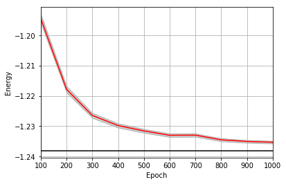
It is assumed that the user has worked through tutorial 3 beforehand. Recall that quantum_ising_chain.py contains the TFIMChainEnergy class that inherits from the Observable module. The exact ground-state energy is -1.2381.

import os.path

import numpy as np
import matplotlib.pyplot as plt

from qucumber.nn_states import PositiveWavefunction
from qucumber.callbacks import ObservableEvaluator

import qucumber.utils.data as data

from quantum_ising_chain import TFIMChainEnergy

train_data = data.load_data(
    os.path.join("..", "Tutorial1_TrainPosRealWavefunction", "tfim1d_data.txt")
)[0]

nv = train_data.shape[-1]
nh = nv

nn_state = PositiveWavefunction(num_visible=nv, num_hidden=nh)

epochs = 1000
pbs = 100  # pos_batch_size
nbs = 200  # neg_batch_size
lr = 0.01
k = 10

log_every = 100

h = 1
num_samples = 10000
burn_in = 100
steps = 100

tfim_energy = TFIMChainEnergy(h)

Now, the ObservableEvaluator can be called. The ObservableEvaluator requires the following arguments.

1. log_every: the frequency of the training evaluators being calculated is controlled by the log_every argument (e.g. log_every = 200 means that the MetricEvaluator will update the user every 200 epochs)
2. A list of Observable objects you would like to reference to evaluate the training (arguments required for generating samples to calculate the observables are keyword arguments placed after the list)

The following additional arguments are needed to calculate the statistics on the generated samples during training (these are the arguments of the statistics function in the Observable module, minus the nn_state argument; this gets passed in as an argument to fit).

• num_samples: the number of samples to generate internally
• num_chains: the number of Markov chains to run in parallel (default = 0)
• burn_in: the number of Gibbs steps to perform before recording any samples (default = 1000)
• steps: the number of Gibbs steps to perform between each sample (default = 1)

The training evaluators can be printed out via the verbose=True statement.

callbacks = [
    ObservableEvaluator(
        log_every,
        [tfim_energy],
        verbose=True,
        num_samples=num_samples,
        burn_in=burn_in,
        steps=steps,
    )
]

nn_state.fit(
    train_data,
    epochs=epochs,
    pos_batch_size=pbs,
    neg_batch_size=nbs,
    lr=lr,
    k=k,
    callbacks=callbacks,
)

Epoch: 100
  TFIMChainEnergy:
    mean: -1.194464     variance: 0.024380      std_error: 0.001561
Epoch: 200
  TFIMChainEnergy:
    mean: -1.217816     variance: 0.012093      std_error: 0.001100
Epoch: 300
  TFIMChainEnergy:
    mean: -1.226431     variance: 0.007242      std_error: 0.000851
Epoch: 400
  TFIMChainEnergy:
    mean: -1.229766     variance: 0.005400      std_error: 0.000735
Epoch: 500
  TFIMChainEnergy:
    mean: -1.231543     variance: 0.004386      std_error: 0.000662
Epoch: 600
  TFIMChainEnergy:
    mean: -1.232977     variance: 0.003655      std_error: 0.000605
Epoch: 700
  TFIMChainEnergy:
    mean: -1.232943     variance: 0.003286      std_error: 0.000573
Epoch: 800
  TFIMChainEnergy:
    mean: -1.234483     variance: 0.002825      std_error: 0.000532
Epoch: 900
  TFIMChainEnergy:
    mean: -1.235027     variance: 0.002327      std_error: 0.000482
Epoch: 1000
  TFIMChainEnergy:
    mean: -1.235285     variance: 0.002064      std_error: 0.000454

The callbacks list returns a list of dictionaries. The mean, standard error and the variance at each epoch can be accessed as follows.

energies = callbacks[0].TFIMChainEnergy.mean
errors = callbacks[0].TFIMChainEnergy.std_error
variance = callbacks[0].TFIMChainEnergy.variance
# Please note that the name of the observable class that the user makes must be what comes after callbacks[0].

A plot of the energy as a function of the training cycle is presented below.

epoch = np.arange(log_every, epochs + 1, log_every)

E0 = -1.2381

ax = plt.axes()
ax.plot(epoch, energies, color="red")
ax.set_xlim(log_every, epochs)
ax.axhline(E0, color="black")
ax.fill_between(epoch, energies - errors, energies + errors, alpha=0.2, color="black")
ax.set_xlabel("Epoch")
ax.set_ylabel("Energy")
ax.grid()