This is a static, non-editable tutorial.

We recommend you install QuCumber if you want to run the examples locally. You can then get an archive file containing the examples from the relevant release here. Alternatively, you can launch an interactive online version, though it may be a bit slow:

Reconstruction of a complex wavefunction¶

In this tutorial, a walkthrough of how to reconstruct a complex wavefunction via training a Restricted Boltzmann Machine (RBM), the neural network behind qucumber, will be presented.

The wavefunction to be reconstructed¶

The simple wavefunction below describing two qubits (coefficients stored in qubits_psi.txt) will be reconstructed.

$\begin{equation} \vert\psi \rangle = \alpha \vert00\rangle + \beta \vert 01\rangle + \gamma \vert10\rangle + \delta \vert11\rangle \end{equation}$

where the exact values of $\alpha, \beta, \gamma$ and $\delta$ used for this tutorial are

$\begin{align} \alpha & = 0.2861 + 0.0539 i \\ \beta & = 0.3687 - 0.3023 i \\ \gamma & = -0.1672 - 0.3529 i \\ \delta & = -0.5659 - 0.4639 i. \end{align}$

The example dataset, qubits_train.txt, comprises of 500 $\sigma$ measurements made in various bases (X, Y and Z). A corresponding file containing the bases for each data point in qubits_train.txt, qubits_train_bases.txt, is also required. As per convention, spins are represented in binary notation with zero and one denoting spin-down and spin-up, respectively.

Using qucumber to reconstruct the wavefunction¶

Imports¶

To begin the tutorial, first import the required Python packages.

In [1]:

import numpy as np
import torch
import matplotlib.pyplot as plt

from qucumber.nn_states import ComplexWavefunction

from qucumber.callbacks import MetricEvaluator

import qucumber.utils.unitaries as unitaries
import qucumber.utils.cplx as cplx

import qucumber.utils.training_statistics as ts
import qucumber.utils.data as data

The Python class ComplexWavefunction contains generic properties of a RBM meant to reconstruct a complex wavefunction, the most notable one being the gradient function required for stochastic gradient descent.

To instantiate a ComplexWavefunction object, one needs to specify the number of visible and hidden units in the RBM. The number of visible units, num_visible, is given by the size of the physical system, i.e. the number of spins or qubits (2 in this case), while the number of hidden units, num_hidden, can be varied to change the expressiveness of the neural network.

Note: The optimal num_hidden : num_visible ratio will depend on the system. For the two-qubit wavefunction described above, good results are yielded when this ratio is 1.

On top of needing the number of visible and hidden units, a ComplexWavefunction object requires the user to input a dictionary containing the unitary operators (2x2) that will be used to rotate the qubits in and out of the computational basis, Z, during the training process. The unitaries utility will take care of creating this dictionary.

The MetricEvaluator class and training_statistics utility are built-in amenities that will allow the user to evaluate the training in real time.

Lastly, the cplx utility allows qucumber to be able to handle complex numbers. Currently, Pytorch does not support complex numbers.

Training¶

To evaluate the training in real time, the fidelity between the true wavefunction of the system and the wavefunction that qucumber reconstructs, $\vert\langle\psi\vert\psi_{RBM}\rangle\vert^2$ , will be calculated along with the Kullback-Leibler (KL) divergence (the RBM’s cost function). First, the training data and the true wavefunction of this system need to be loaded using the data utility.

In [2]:

train_path = "qubits_train.txt"
train_bases_path = "qubits_train_bases.txt"
psi_path = "qubits_psi.txt"
bases_path = "qubits_bases.txt"

train_samples, true_psi, train_bases, bases = data.load_data(
    train_path, psi_path, train_bases_path, bases_path
)

The file qubits_bases.txt contains every unique basis in the qubits_train_bases.txt file. Calculation of the full KL divergence in every basis requires the user to specify each unique basis.

As previouosly mentioned, a ComplexWavefunction object requires a dictionary that contains the unitariy operators that will be used to rotate the qubits in and out of the computational basis, Z, during the training process. In the case of the provided dataset, the unitaries required are the well-known $H$ , and $K$ gates. The dictionary needed can be created with the following command.

In [3]:

unitary_dict = unitaries.create_dict()
# unitary_dict = unitaries.create_dict(unitary_name=torch.tensor([[real part],
#                                                                 [imaginary part]],
#                                                                 dtype=torch.double)

If the user wishes to add their own unitary operators from their experiment to unitary_dict, uncomment the block above. When unitaries.create_dict() is called, it will contain the identity and the $H$ and $K$ gates by default with the keys “Z”, “X” and “Y”, respectively.

The number of visible units in the RBM is equal to the number of qubits. The number of hidden units will also be taken to be the number of visible units.

In [4]:

nv = train_samples.shape[-1]
nh = nv

nn_state = ComplexWavefunction(
    num_visible=nv, num_hidden=nh, unitary_dict=unitary_dict, gpu=False
)
# nn_state = ComplexWavefunction(num_visible=nv, num_hidden=nh, unitary_dict=unitary_dict)

By default, qucumber will attempt to run on a GPU if one is available (if one is not available, qucumber will default to CPU). If one wishes to run qucumber on a CPU, add the flag “gpu = False” in the ComplexWavefunction object instantiation. Uncomment the line above to run this tutorial on a GPU.

Now the hyperparameters of the training process can be specified.

epochs: the total number of training cycles that will be performed (default = 100)
pos_batch_size: the number of data points used in the positive phase of the gradient (default = 100)
neg_batch_size: the number of data points used in the negative phase of the gradient (default = pos_batch_size)
k: the number of contrastive divergence steps (default = 1)
lr: the learning rate (default = 0.001)

Note: For more information on the hyperparameters above, it is strongly encouraged that the user to read through the brief, but thorough theory document on RBMs. One does not have to specify these hyperparameters, as their default values will be used without the user overwriting them. It is recommended to keep with the default values until the user has a stronger grasp on what these hyperparameters mean. The quality and the computational efficiency of the training will highly depend on the choice of hyperparameters. As such, playing around with the hyperparameters is almost always necessary.

The two-qubit example in this tutorial should be extremely easy to train, regardless of the choice of hyperparameters. However, the hyperparameters below will be used.

In [5]:

epochs = 80
pbs = 50  # pos_batch_size
nbs = 10  # neg_batch_size
lr = 0.1
k = 5

For evaluating the training in real time, the MetricEvaluator will be called to calculate the training evaluators every 10 epochs. The MetricEvaluator requires the following arguments.

log_every: the frequency of the training evaluators being calculated is controlled by the log_every argument (e.g. log_every = 200 means that the MetricEvaluator will update the user every 200 epochs)
A dictionary of functions you would like to reference to evaluate the training (arguments required for these functions are keyword arguments placed after the dictionary)

The following additional arguments are needed to calculate the fidelity and KL divergence in the training_statistics utility.

target_psi (the true wavefunction of the system)
space (the hilbert space of the system)

The training evaluators can be printed out via the verbose=True statement.

Although the fidelity and KL divergence are excellent training evaluators, they are not practical to calculate in most cases; the user may not have access to the target wavefunction of the system, nor may generating the hilbert space of the system be computationally feasible. However, evaluating the training in real time is extremely convenient.

Any custom function that the user would like to use to evaluate the training can be given to the MetricEvaluator, thus avoiding having to calculate fidelity and/or KL divergence. As an example, functions that calculate the the norm of each of the reconstructed wavefunction’s coefficients are presented. Any custom function given to MetricEvaluator must take the neural-network state (in this case, the ComplexWavefunction object) and keyword arguments. Although the given example requires the hilbert space to be computed, the scope of the MetricEvaluator’s ability to be able to handle any function should still be evident.

In [6]:

def alpha(nn_state, space, **kwargs):
    rbm_psi = nn_state.psi(space)
    normalization = nn_state.compute_normalization(space).sqrt_()
    alpha_ = cplx.norm(
        torch.tensor([rbm_psi[0][0], rbm_psi[1][0]], device=nn_state.device)
        / normalization
    )

    return alpha_


def beta(nn_state, space, **kwargs):
    rbm_psi = nn_state.psi(space)
    normalization = nn_state.compute_normalization(space).sqrt_()
    beta_ = cplx.norm(
        torch.tensor([rbm_psi[0][1], rbm_psi[1][1]], device=nn_state.device)
        / normalization
    )

    return beta_


def gamma(nn_state, space, **kwargs):
    rbm_psi = nn_state.psi(space)
    normalization = nn_state.compute_normalization(space).sqrt_()
    gamma_ = cplx.norm(
        torch.tensor([rbm_psi[0][2], rbm_psi[1][2]], device=nn_state.device)
        / normalization
    )

    return gamma_


def delta(nn_state, space, **kwargs):
    rbm_psi = nn_state.psi(space)
    normalization = nn_state.compute_normalization(space).sqrt_()
    delta_ = cplx.norm(
        torch.tensor([rbm_psi[0][3], rbm_psi[1][3]], device=nn_state.device)
        / normalization
    )

    return delta_

Now the hilbert space of the system must be generated for the fidelity and KL divergence and the dictionary of functions the user would like to compute every “log_every” epochs must be given to the MetricEvaluator.

In [7]:

log_every = 10
space = nn_state.generate_hilbert_space(nv)

callbacks = [
    MetricEvaluator(
        log_every,
        {
            "Fidelity": ts.fidelity,
            "KL": ts.KL,
            "normα": alpha,
            "normβ": beta,
            "normγ": gamma,
            "normδ": delta,
        },
        target_psi=true_psi,
        bases=bases,
        verbose=True,
        space=space,
    )
]

Now the training can begin. The ComplexWavefunction object has a property called fit which takes care of this.

In [8]:

nn_state.fit(
    train_samples,
    epochs=epochs,
    pos_batch_size=pbs,
    neg_batch_size=nbs,
    lr=lr,
    k=k,
    input_bases=train_bases,
    callbacks=callbacks,
)

Epoch: 10       Fidelity = 0.584157     KL = 0.239528   normα = 0.203017        normβ = 0.333242        normγ = 0.440140        normδ = 0.808709
Epoch: 20       Fidelity = 0.900338     KL = 0.046861   normα = 0.284082        normβ = 0.468427        normγ = 0.408342        normδ = 0.730158
Epoch: 30       Fidelity = 0.964009     KL = 0.022833   normα = 0.284898        normβ = 0.489092        normγ = 0.390978        normδ = 0.725781
Epoch: 40       Fidelity = 0.979635     KL = 0.015013   normα = 0.286033        normβ = 0.462681        normγ = 0.415928        normδ = 0.728777
Epoch: 50       Fidelity = 0.978498     KL = 0.017450   normα = 0.264300        normβ = 0.413593        normγ = 0.439953        normδ = 0.752016
Epoch: 60       Fidelity = 0.983162     KL = 0.013628   normα = 0.284534        normβ = 0.433017        normγ = 0.443165        normδ = 0.731533
Epoch: 70       Fidelity = 0.989934     KL = 0.009804   normα = 0.265790        normβ = 0.484255        normγ = 0.378505        normδ = 0.742689
Epoch: 80       Fidelity = 0.990302     KL = 0.009240   normα = 0.255228        normβ = 0.458123        normγ = 0.389683        normδ = 0.757053

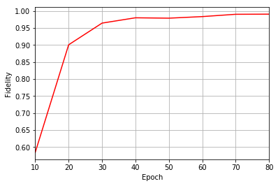
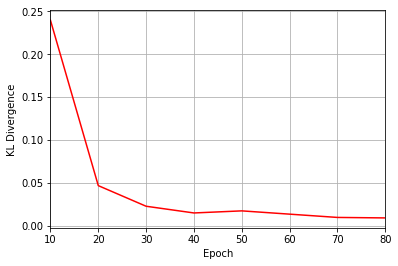
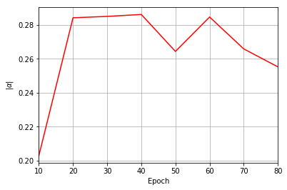
All of these training evaluators can be accessed after the training has completed, as well. The code below shows this, along with plots of each training evaluator versus the training cycle number (epoch).

In [9]:

fidelities = callbacks[0].Fidelity
KLs = callbacks[0].KL
coeffs = callbacks[0].normα
# Please note that the key given to the *MetricEvaluator* must be what comes after callbacks[0].
epoch = np.arange(log_every, epochs + 1, log_every)

plt.figure(1)
ax1 = plt.axes()
ax1.grid()
ax1.set_xlim(log_every, epochs)
ax1.set_xlabel("Epoch")
ax1.set_ylabel("Fidelity")
ax1.plot(epoch, fidelities, color="r")

plt.figure(2)
ax2 = plt.axes()
ax2.grid()
ax2.set_xlim(log_every, epochs)
ax2.set_xlabel("Epoch")
ax2.set_ylabel("KL Divergence")
ax2.plot(epoch, KLs, color="r")

plt.figure(3)
ax3 = plt.axes()
ax3.grid()
ax3.set_xlim(log_every, epochs)
ax3.set_xlabel("Epoch")
ax3.set_ylabel(r"$\vert\alpha\vert$")
ax3.plot(epoch, coeffs, color="r")

Out[9]:

[<matplotlib.lines.Line2D at 0x7f216c73b940>]

../../_images/_examples_Tutorial2_TrainComplexWavefunction_tutorial_qubits_17_1.png

../../_images/_examples_Tutorial2_TrainComplexWavefunction_tutorial_qubits_17_2.png

../../_images/_examples_Tutorial2_TrainComplexWavefunction_tutorial_qubits_17_3.png

It should be noted that one could have just ran nn_state.fit(train_samples) and just used the default hyperparameters and no training evaluators.

At the end of the training process, the network parameters (the weights, visible biases and hidden biases) are stored in the ComplexWavefunction object. One can save them to a pickle file, which will be called saved_params.pt, with the following command.

In [10]:

nn_state.save("saved_params.pt")

This saves the weights, visible biases and hidden biases as torch tensors with the following keys: “weights”, “visible_bias”, “hidden_bias”.