This is a static, non-editable tutorial.
We recommend you install QuCumber if you want to run the examples locally.
You can then get an archive file containing the examples from the relevant release
here.
Alternatively, you can launch an interactive online version, though it may be a bit slow:
![]()
Reconstruction of a density matrix
In this tutorial, a walkthrough of how to reconstruct a density matrix via training a pair of modified Restricted Boltzmann Machines is presented
The density matrix to be reconstructed
The density matrix that will be be reconstructed is the density matrix associated with the 2-qubit W state

so that

with global depolarization probability  such that

where  is the identity matrix, representing the maximally mixed state.
The example dataset, N2_W_state_100_samples_data.txt, is comprised of 900  measurements, 100 in each of the
  permutations of two of the bases X, Y and Z. A corresponding file containing the bases for each data point,
 N2_W_state_100_samples_bases.txt, is also required.
In this tutorial is also included versions with 1000 measurements in each basis, to illustrate the improvements to reconstruction fidelity of a larger data set. The measurements and bases are stored in N2_W_state_1000_samples_data.txt, and N2_W_state_1000_samples_bases.txt respectively.
The set of all 3^2 bases in which measurements are made is stored in N2_IC_bases.txt. Finally, the real and imaginary parts of the matrix are stored in N2_W_state_target_real.txt and N2_W_state_target_imag.txt respectively. As per convention, spins are represented in binary notation with zero and one denoting spin-up and spin-down, respectively.
Using QuCumber to reconstruct the density matrix
Imports
To begin the tutorial, first import the required Python packages.
[1]:
import numpy as np
import matplotlib.pyplot as plt

import torch

from qucumber.nn_states import DensityMatrix

from qucumber.callbacks import MetricEvaluator
import qucumber.utils.unitaries as unitaries

import qucumber.utils.training_statistics as ts
import qucumber.utils.data as data
import qucumber

# set random seed on cpu but not gpu, since we won't use gpu for this tutorial
qucumber.set_random_seed(1234, cpu=True, gpu=False)
The Python class DensityMatrix contains the properties of an RBM needed to reconstruct the density matrix, as demonstrated in this paper here.
To instantiate a DensityMatrix object, one needs to specify the number of visible, hidden and auxiliary units in the RBM. The number of visible units, num_visible, is given by the size of the physical system, i.e. the number of spins or qubits (2 in this case). On the other hand, the number of hidden units, num_hidden, can be varied to change the expressiveness of the neural network, and the number of auxiliary units, num_aux, can be varied depending on the extent of purification
required of the system.
On top of needing the number of visible, hidden and auxiliary units, a DensityMatrix object requires the user to input a dictionary containing the unitary operators (2x2) that will be used to rotate the qubits in and out of the computational basis, Z, during the training process. The unitaries utility will take care of creating this dictionary.
The MetricEvaluator class and training_statistics utility are built-in amenities that will allow the user to evaluate the training in real time.
Training
To evaluate the training in real time, the fidelity between the true wavefunction of the system and the wavefunction that QuCumber reconstructs,

will be calculated along with the Kullback-Leibler (KL) divergence (the RBM’s cost function). First, the training data and the true wavefunction of this system need to be loaded using the data utility.
[2]:
train_path = "N2_W_state_100_samples_data.txt"
train_bases_path = "N2_W_state_100_samples_bases.txt"
matrix_path_real = "N2_W_state_target_real.txt"
matrix_path_imag = "N2_W_state_target_imag.txt"
bases_path = "N2_IC_bases.txt"


train_samples, true_matrix, train_bases, bases = data.load_data_DM(
    train_path, matrix_path_real, matrix_path_imag, train_bases_path, bases_path
)
The file N2_IC_bases.txt contains every unique basis in the N2_W_state_100_samples_bases.txt file. Calculation of the full KL divergence in every basis requires the user to specify each unique basis.
As previously mentioned, a DensityMatrix object requires a dictionary that contains the unitary operators that will be used to rotate the qubits in and out of the computational basis, Z, during the training process. In the case of the provided dataset, the unitaries required are the well-known  , and
, and  gates. The dictionary needed can be created with the following command.
[3]:
unitary_dict = unitaries.create_dict()
# unitary_dict = unitaries.create_dict(unitary_name=torch.tensor([[real part],
#                                                                 [imaginary part]],
#                                                                 dtype=torch.double)
If the user wishes to add their own unitary operators from their experiment to unitary_dict, uncomment the block above. When unitaries.create_dict() is called, it will contain the identity and the and gates by default under the keys “Z”, “X” and “Y”, respectively.
The number of visible units in the RBM is equal to the number of qubits. The number of hidden units will also be taken to be the number of visible units.
[4]:
nv = train_samples.shape[-1]
nh = na = nv

nn_state = DensityMatrix(
    num_visible=nv, num_hidden=nh, num_aux=na, unitary_dict=unitary_dict, gpu=False
)
The number of visible, hidden, and auxiliary units must now be specified. These are given by nv, nh and na respectively. The number of visible units is equal to the size of the system. The hidden and auxiliary units are hyperparameters that must be provided by the user. With these, a DensityMatrix object can be instantiated.
Now the hyperparameters of the training process can be specified.
epochs: the total number of training cycles that will be performed (default = 100)pos_batch_size: the number of data points used in the positive phase of the gradient (default = 100)neg_batch_size: the number of data points used in the negative phase of the gradient (default =pos_batch_size)k: the number of contrastive divergence steps (default = 1)lr: coefficient that scales the default value of the (non-constant) learning rate of the Adadelta algorithm (default = 1)
Extra hyperparameters that we will be passing to the learning rate scheduler: 6. lr_drop_epochs: the number of epochs after which to decay the learning rate by lr_drop_factor 7. lr_drop_factor: the factor by which the learning rate drops at lr_drop_epoch or all epochs in lr_drop_epoch if it is a list
Set lr_drop_factor to 1.0 to maintain constant “base” learning rate for Adadelta optimization. The choice shown here is optimized for this tutorial, but can (and should) be varied according to each instance
Note: For more information on the hyperparameters above, it is strongly encouraged that the user to read through the brief, but thorough theory document on RBMs. One does not have to specify these hyperparameters, as their default values will be used without the user overwriting them. It is recommended to keep with the default values until the user has a stronger grasp on what these hyperparameters mean. The quality and the computational efficiency of the training will highly depend on the choice of hyperparameters. As such, playing around with the hyperparameters is almost always necessary.
[5]:
epochs = 500
pbs = 100  # pos_batch_size
nbs = pbs  # neg_batch_size
lr = 10
k = 10
lr_drop_epoch = 125
lr_drop_factor = 0.5
For evaluating the training in real time, the MetricEvaluator will be called to calculate the training evaluators every period epochs. The MetricEvaluator requires the following arguments.
period: the frequency of the training evaluators being calculated (e.g.period=200means that theMetricEvaluatorwill compute the desired metrics every 200 epochs)A dictionary of functions you would like to reference to evaluate the training (arguments required for these functions are keyword arguments placed after the dictionary)
The following additional arguments are needed to calculate the fidelity and KL divergence in the training_statistics utility.
target_matrix(the true density matrix of the system)space(the entire Hilbert space of the system)
The training evaluators can be printed out via the verbose=True statement.
Although the fidelity and KL divergence are excellent training evaluators, they are not practical to calculate in most cases; the user may not have access to the target wavefunction of the system, nor may generating the Hilbert space of the system be computationally feasible. However, evaluating the training in real time is extremely convenient.
Any custom function that the user would like to use to evaluate the training can be given to the MetricEvaluator, thus avoiding having to calculate fidelity and/or KL divergence. As an example, a function to compute the partition function of the current density matrix is presented. Any custom function given to MetricEvaluator must take the neural-network state (in this case, the Density object) and keyword arguments. Although the given example requires the Hilbert space to be
computed, the scope of the MetricEvaluator’s ability to be able to handle any function should still be evident.
[6]:
def partition(nn_state, space, **kwargs):
    return nn_state.rbm_am.partition(space)
Now the Hilbert space of the system must be generated for the fidelity and KL divergence and the dictionary of functions the user would like to compute every period epochs must be given to the MetricEvaluator.
[7]:
period = 25
space = nn_state.generate_hilbert_space()

callbacks = [
    MetricEvaluator(
        period,
        {
            "Fidelity": ts.fidelity,
            "KL": ts.KL,
            # "Partition Function": partition,
        },
        target=true_matrix,
        bases=bases,
        verbose=True,
        space=space,
    )
]
Now the training can begin. The DensityMatrix object has a function called fit which takes care of this.
[8]:
nn_state.fit(
    data=train_samples,
    input_bases=train_bases,
    epochs=epochs,
    pos_batch_size=pbs,
    neg_batch_size=nbs,
    lr=lr,
    k=k,
    bases=bases,
    callbacks=callbacks,
    time=True,
    optimizer=torch.optim.Adadelta,
    scheduler=torch.optim.lr_scheduler.StepLR,
    scheduler_args={"step_size": lr_drop_epoch, "gamma": lr_drop_factor},
)
Epoch: 25       Fidelity = 0.863061     KL = 0.050122
Epoch: 50       Fidelity = 0.946054     KL = 0.013152
Epoch: 75       Fidelity = 0.950760     KL = 0.016754
Epoch: 100      Fidelity = 0.957204     KL = 0.015601
Epoch: 125      Fidelity = 0.960522     KL = 0.013925
Epoch: 150      Fidelity = 0.957411     KL = 0.017446
Epoch: 175      Fidelity = 0.961068     KL = 0.013377
Epoch: 200      Fidelity = 0.966589     KL = 0.010754
Epoch: 225      Fidelity = 0.951836     KL = 0.017970
Epoch: 250      Fidelity = 0.960255     KL = 0.012612
Epoch: 275      Fidelity = 0.961232     KL = 0.012477
Epoch: 300      Fidelity = 0.963946     KL = 0.011832
Epoch: 325      Fidelity = 0.959750     KL = 0.013571
Epoch: 350      Fidelity = 0.965108     KL = 0.011095
Epoch: 375      Fidelity = 0.965353     KL = 0.011048
Epoch: 400      Fidelity = 0.963568     KL = 0.011941
Epoch: 425      Fidelity = 0.966334     KL = 0.011148
Epoch: 450      Fidelity = 0.965549     KL = 0.011321
Epoch: 475      Fidelity = 0.965054     KL = 0.011573
Epoch: 500      Fidelity = 0.965568     KL = 0.010963
Total time elapsed during training: 175.240 s
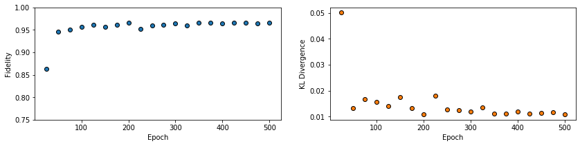
All of these training evaluators can be accessed after the training has completed, as well. The code below shows this, along with plots of each training evaluator versus the training cycle number (epoch).
[9]:
fidelities = callbacks[0]["Fidelity"]
KLs = callbacks[0]["KL"]
epoch = np.arange(period, epochs + 1, period)
[10]:
fig, axs = plt.subplots(nrows=1, ncols=2, figsize=(14, 3))
ax = axs[0]
ax.plot(epoch, fidelities, "o", color="C0", markeredgecolor="black")
ax.set_ylabel(r"Fidelity")
ax.set_xlabel(r"Epoch")
ax.set_ylim(0.75, 1.00)

ax = axs[1]
ax.plot(epoch, KLs, "o", color="C1", markeredgecolor="black")
ax.set_ylabel(r"KL Divergence")
ax.set_xlabel(r"Epoch")
[10]:
Text(0.5, 0, 'Epoch')
This saves the weights, and biases of the two internal RBMs as dictionaries containing torch tensors.
[11]:
nn_state.save("saved_params_W_state.pt")