This is a static, non-editable tutorial.

We recommend you install QuCumber if you want to run the examples locally. You can then get an archive file containing the examples from the relevant release here. Alternatively, you can launch an interactive online version, though it may be a bit slow:

Reconstruction of a positive-real wavefunction¶

This tutorial shows how to reconstruct a positive-real wavefunction via training a Restricted Boltzmann Machine (RBM), the neural network behind QuCumber. The data used for training are $\sigma^{z}$ measurements from a one-dimensional transverse-field Ising model (TFIM) with 10 sites at its critical point.

Transverse-field Ising model¶

The example dataset, located in tfim1d_data.txt, comprises 10,000 $\sigma^{z}$ measurements from a one-dimensional TFIM with 10 sites at its critical point. The Hamiltonian for the TFIM is given by

$\begin{equation} \mathcal{H} = -J\sum_i \sigma^z_i \sigma^z_{i+1} - h \sum_i \sigma^x_i \end{equation}$

where $\sigma^{z}_i$ is the conventional spin-1/2 Pauli operator on site $i$ . At the critical point, $J=h=1$ . By convention, spins are represented in binary notation with zero and one denoting the states spin-down and spin-up, respectively.

Using QuCumber to reconstruct the wavefunction¶

Imports¶

To begin the tutorial, first import the required Python packages.

[1]:

import numpy as np
import matplotlib.pyplot as plt

from qucumber.nn_states import PositiveWaveFunction
from qucumber.callbacks import MetricEvaluator

import qucumber.utils.training_statistics as ts
import qucumber.utils.data as data

The Python class PositiveWaveFunction contains generic properties of a RBM meant to reconstruct a positive-real wavefunction, the most notable one being the gradient function required for stochastic gradient descent.

To instantiate a PositiveWaveFunction object, one needs to specify the number of visible and hidden units in the RBM. The number of visible units, num_visible, is given by the size of the physical system, i.e. the number of spins or qubits (10 in this case), while the number of hidden units, num_hidden, can be varied to change the expressiveness of the neural network.

Note: The optimal num_hidden : num_visible ratio will depend on the system. For the TFIM, having this ratio be equal to 1 leads to good results with reasonable computational effort.

Training¶

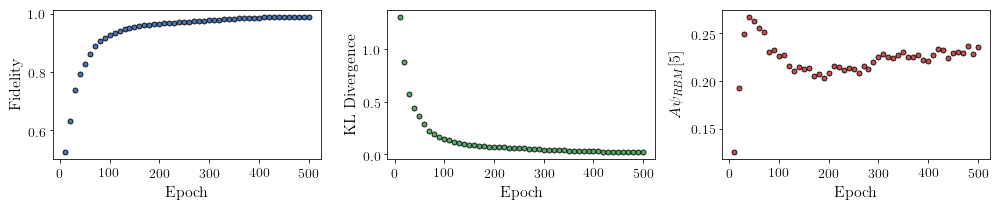
To evaluate the training in real time, we compute the fidelity between the true ground-state wavefunction of the system and the wavefunction that QuCumber reconstructs, $\vert\langle\psi\vert\psi_{RBM}\rangle\vert^2$ , along with the Kullback-Leibler (KL) divergence (the RBM’s cost function). As will be shown below, any custom function can be used to evaluate the training.

First, the training data and the true wavefunction of this system must be loaded using the data utility.

[2]:

psi_path = "tfim1d_psi.txt"
train_path = "tfim1d_data.txt"
train_data, true_psi = data.load_data(train_path, psi_path)

As previously mentioned, to instantiate a PositiveWaveFunction object, one needs to specify the number of visible and hidden units in the RBM; we choose them to be equal.

[3]:

nv = train_data.shape[-1]
nh = nv

nn_state = PositiveWaveFunction(num_visible=nv, num_hidden=nh)
# nn_state = PositiveWaveFunction(num_visible=nv, num_hidden=nh, gpu = False)

By default, QuCumber will attempt to run on a GPU, and default to CPU if GPU is not available. To run QuCumber on a CPU, add the flag gpu=False in the PositiveWaveFunction object instantiation (i.e. uncomment the line above).

Now we specify the hyperparameters of the training process:

epochs: the total number of training cycles that will be performed (default = 100)
pbs (pos_batch_size): the number of data points used in the positive phase of the gradient (default = 100)
nbs (neg_batch_size): the number of data points used in the negative phase of the gradient (default = 100)
k: the number of contrastive divergence steps (default = 1)
lr: the learning rate (default = 0.001)

Note: For more information on the hyperparameters above, it is strongly encouraged that the user to read through the brief, but thorough theory document on RBMs located in the QuCumber documentation. One does not have to specify these hyperparameters, as their default values will be used without the user overwriting them. It is recommended to keep with the default values until the user has a stronger grasp on what these hyperparameters mean. The quality and the computational efficiency of the training will highly depend on the choice of hyperparameters. As such, playing around with the hyperparameters is almost always necessary.

For the TFIM with 10 sites, the following hyperparameters give excellent results:

[4]:

epochs = 500
pbs = 100
nbs = pbs
lr = 0.01
k = 10

For evaluating the training in real time, the MetricEvaluator is called every 100 epochs in order to calculate the training evaluators. The MetricEvaluator requires the following arguments:

period: the frequency of the training evaluators being calculated (e.g. period=100 means that the MetricEvaluator will do an evaluation every 100 epochs)
A dictionary of functions you would like to reference to evaluate the training (arguments required for these functions are keyword arguments placed after the dictionary)

The following additional arguments are needed to calculate the fidelity and KL divergence in the training_statistics utility:

target_psi: the true wavefunction of the system
space: the Hilbert space of the system

The training evaluators can be printed out via the verbose=True statement.

Although the fidelity and KL divergence are excellent training evaluators, they are not practical to calculate in most cases; the user may not have access to the target wavefunction of the system, nor may generating the Hilbert space of the system be computationally feasible. However, evaluating the training in real time is extremely convenient.

Any custom function that the user would like to use to evaluate the training can be given to the MetricEvaluator, thus avoiding having to calculate fidelity and/or KL divergence. Any custom function given to MetricEvaluator must take the neural-network state (in this case, the PositiveWaveFunction object) and keyword arguments. As an example, we define a custom function psi_coefficient, which is the fifth coefficient of the reconstructed wavefunction multiplied by a parameter $A$ .

[5]:

def psi_coefficient(nn_state, space, A, **kwargs):
    norm = nn_state.compute_normalization(space).sqrt_()
    return A * nn_state.psi(space)[0][4] / norm

Now the Hilbert space of the system can be generated for the fidelity and KL divergence.

[6]:

period = 10
space = nn_state.generate_hilbert_space(nv)

Now the training can begin. The PositiveWaveFunction object has a property called fit which takes care of this. MetricEvaluator must be passed to the fit function in a list (callbacks).

[7]:

callbacks = [
    MetricEvaluator(
        period,
        {"Fidelity": ts.fidelity, "KL": ts.KL, "A_Ψrbm_5": psi_coefficient},
        target_psi=true_psi,
        verbose=True,
        space=space,
        A=3.0,
    )
]

nn_state.fit(
    train_data,
    epochs=epochs,
    pos_batch_size=pbs,
    neg_batch_size=nbs,
    lr=lr,
    k=k,
    callbacks=callbacks,
)

Epoch: 10       Fidelity = 0.526148     KL = 1.310731   A_Ψrbm_5 = 0.125463
Epoch: 20       Fidelity = 0.631814     KL = 0.875887   A_Ψrbm_5 = 0.193193
Epoch: 30       Fidelity = 0.736986     KL = 0.577408   A_Ψrbm_5 = 0.249697
Epoch: 40       Fidelity = 0.794626     KL = 0.445550   A_Ψrbm_5 = 0.267554
Epoch: 50       Fidelity = 0.828487     KL = 0.363523   A_Ψrbm_5 = 0.263156
Epoch: 60       Fidelity = 0.861033     KL = 0.284768   A_Ψrbm_5 = 0.255909
Epoch: 70       Fidelity = 0.888133     KL = 0.226607   A_Ψrbm_5 = 0.251317
Epoch: 80       Fidelity = 0.904473     KL = 0.191903   A_Ψrbm_5 = 0.230342
Epoch: 90       Fidelity = 0.916896     KL = 0.168523   A_Ψrbm_5 = 0.232834
Epoch: 100      Fidelity = 0.925543     KL = 0.151414   A_Ψrbm_5 = 0.226578
Epoch: 110      Fidelity = 0.933069     KL = 0.136249   A_Ψrbm_5 = 0.227657
Epoch: 120      Fidelity = 0.939533     KL = 0.122066   A_Ψrbm_5 = 0.216086
Epoch: 130      Fidelity = 0.945398     KL = 0.109634   A_Ψrbm_5 = 0.210336
Epoch: 140      Fidelity = 0.950329     KL = 0.099964   A_Ψrbm_5 = 0.214536
Epoch: 150      Fidelity = 0.954255     KL = 0.092397   A_Ψrbm_5 = 0.212398
Epoch: 160      Fidelity = 0.957539     KL = 0.086165   A_Ψrbm_5 = 0.213869
Epoch: 170      Fidelity = 0.959890     KL = 0.081415   A_Ψrbm_5 = 0.205124
Epoch: 180      Fidelity = 0.961762     KL = 0.077955   A_Ψrbm_5 = 0.207600
Epoch: 190      Fidelity = 0.963395     KL = 0.075018   A_Ψrbm_5 = 0.203214
Epoch: 200      Fidelity = 0.965103     KL = 0.071877   A_Ψrbm_5 = 0.207948
Epoch: 210      Fidelity = 0.966435     KL = 0.069428   A_Ψrbm_5 = 0.216086
Epoch: 220      Fidelity = 0.967274     KL = 0.067780   A_Ψrbm_5 = 0.215082
Epoch: 230      Fidelity = 0.968685     KL = 0.064706   A_Ψrbm_5 = 0.211092
Epoch: 240      Fidelity = 0.969841     KL = 0.062323   A_Ψrbm_5 = 0.213523
Epoch: 250      Fidelity = 0.971052     KL = 0.059850   A_Ψrbm_5 = 0.212783
Epoch: 260      Fidelity = 0.971965     KL = 0.057842   A_Ψrbm_5 = 0.208115
Epoch: 270      Fidelity = 0.973736     KL = 0.054289   A_Ψrbm_5 = 0.215748
Epoch: 280      Fidelity = 0.974085     KL = 0.053346   A_Ψrbm_5 = 0.212171
Epoch: 290      Fidelity = 0.976066     KL = 0.049299   A_Ψrbm_5 = 0.219986
Epoch: 300      Fidelity = 0.977303     KL = 0.046733   A_Ψrbm_5 = 0.225259
Epoch: 310      Fidelity = 0.978261     KL = 0.044790   A_Ψrbm_5 = 0.228821
Epoch: 320      Fidelity = 0.979351     KL = 0.042555   A_Ψrbm_5 = 0.225733
Epoch: 330      Fidelity = 0.980212     KL = 0.040565   A_Ψrbm_5 = 0.223765
Epoch: 340      Fidelity = 0.981664     KL = 0.037660   A_Ψrbm_5 = 0.226980
Epoch: 350      Fidelity = 0.982528     KL = 0.035918   A_Ψrbm_5 = 0.230829
Epoch: 360      Fidelity = 0.983351     KL = 0.034181   A_Ψrbm_5 = 0.224962
Epoch: 370      Fidelity = 0.984213     KL = 0.032504   A_Ψrbm_5 = 0.225617
Epoch: 380      Fidelity = 0.984872     KL = 0.031177   A_Ψrbm_5 = 0.227120
Epoch: 390      Fidelity = 0.985186     KL = 0.030594   A_Ψrbm_5 = 0.222515
Epoch: 400      Fidelity = 0.985662     KL = 0.029606   A_Ψrbm_5 = 0.220782
Epoch: 410      Fidelity = 0.986466     KL = 0.028079   A_Ψrbm_5 = 0.227727
Epoch: 420      Fidelity = 0.986970     KL = 0.027100   A_Ψrbm_5 = 0.233300
Epoch: 430      Fidelity = 0.987040     KL = 0.026978   A_Ψrbm_5 = 0.232759
Epoch: 440      Fidelity = 0.987675     KL = 0.025714   A_Ψrbm_5 = 0.224514
Epoch: 450      Fidelity = 0.988244     KL = 0.024636   A_Ψrbm_5 = 0.229669
Epoch: 460      Fidelity = 0.988569     KL = 0.023975   A_Ψrbm_5 = 0.230897
Epoch: 470      Fidelity = 0.988666     KL = 0.023802   A_Ψrbm_5 = 0.229378
Epoch: 480      Fidelity = 0.988781     KL = 0.023565   A_Ψrbm_5 = 0.236488
Epoch: 490      Fidelity = 0.989243     KL = 0.022694   A_Ψrbm_5 = 0.228858
Epoch: 500      Fidelity = 0.988991     KL = 0.023196   A_Ψrbm_5 = 0.235301

All of these training evaluators can be accessed after the training has completed. The code below shows this, along with plots of each training evaluator as a function of epoch (training cycle number).

[8]:

# Note that the key given to the *MetricEvaluator* must be
# what comes after callbacks[0].
fidelities = callbacks[0].Fidelity

# Alternatively, we can use the usual dictionary/list subsripting
# syntax. This is useful in cases where the name of the
# metric contains special characters or spaces.
KLs = callbacks[0]["KL"]
coeffs = callbacks[0]["A_Ψrbm_5"]

epoch = np.arange(period, epochs + 1, period)

[9]:

# Some parameters to make the plots look nice
params = {
    "text.usetex": True,
    "font.family": "serif",
    "legend.fontsize": 14,
    "figure.figsize": (10, 3),
    "axes.labelsize": 16,
    "xtick.labelsize": 14,
    "ytick.labelsize": 14,
    "lines.linewidth": 2,
    "lines.markeredgewidth": 0.8,
    "lines.markersize": 5,
    "lines.marker": "o",
    "patch.edgecolor": "black",
}
plt.rcParams.update(params)
plt.style.use("seaborn-deep")

[10]:

# Plotting
fig, axs = plt.subplots(nrows=1, ncols=3, figsize=(14, 3))
ax = axs[0]
ax.plot(epoch, fidelities, "o", color="C0", markeredgecolor="black")
ax.set_ylabel(r"Fidelity")
ax.set_xlabel(r"Epoch")

ax = axs[1]
ax.plot(epoch, KLs, "o", color="C1", markeredgecolor="black")
ax.set_ylabel(r"KL Divergence")
ax.set_xlabel(r"Epoch")

ax = axs[2]
ax.plot(epoch, coeffs, "o", color="C2", markeredgecolor="black")
ax.set_ylabel(r"$A\psi_{RBM}[5]$")
ax.set_xlabel(r"Epoch")

plt.tight_layout()
plt.savefig("fid_KL.pdf")
plt.show()

../../_images/_examples_Tutorial1_TrainPosRealWaveFunction_tutorial_quantum_ising_17_0.png

It should be noted that one could have just ran nn_state.fit(train_samples), which uses the default hyperparameters and no training evaluators.

To demonstrate how important it is to find the optimal hyperparameters for a certain system, restart this notebook and comment out the original fit statement, then uncomment and run the cell below.

[11]:

# nn_state.fit(train_samples)

Using the non-default hyperparameters yielded a fidelity of approximately $0.989$ , while the default hyperparameters yield approximately $0.523$ !

The trained RBM’s parameters are saved to a pickle file with the name saved_params.pt for future use in other tutorials:

[12]:

nn_state.save("saved_params.pt")

This saves the weights, visible biases and hidden biases as torch tensors with the following keys: “weights”, “visible_bias”, “hidden_bias”.