This is a static, non-editable tutorial.

We recommend you install QuCumber if you want to run the examples locally. You can then get an archive file containing the examples from the relevant release here. Alternatively, you can launch an interactive online version, though it may be a bit slow:

Reconstruction of a positive-real wavefunction¶

In this tutorial, a walkthrough of how to reconstruct a positive-real wavefunction via training a Restricted Boltzmann Machine (RBM), the neural network behind QuCumber, will be presented. The data used for training will be $\sigma^{z}$ measurements from a one-dimensional transverse-field Ising model (TFIM) with 10 sites at its critical point.

Transverse-field Ising model¶

The example dataset, located in tfim1d_data.txt, comprises of 10,000 $\sigma^{z}$ measurements from a one-dimensional transverse-field Ising model (TFIM) with 10 sites at its critical point. The Hamiltonian for the transverse-field Ising model (TFIM) is given by

$\begin{equation} \mathcal{H} = -J\sum_i \sigma^z_i \sigma^z_{i+1} - h \sum_i \sigma^x_i \end{equation}$

where $\sigma^{z}_i$ is the conventional spin-1/2 Pauli operator on site $i$ . At the critical point, $J=h=1$ . As per convention, spins are represented in binary notation with zero and one denoting spin-down and spin-up, respectively.

Using QuCumber to reconstruct the wavefunction¶

Imports¶

To begin the tutorial, first import the required Python packages.

[1]:

import numpy as np
import matplotlib.pyplot as plt

from qucumber.nn_states import PositiveWaveFunction
from qucumber.callbacks import MetricEvaluator

import qucumber.utils.training_statistics as ts
import qucumber.utils.data as data

The Python class PositiveWaveFunction contains generic properties of a RBM meant to reconstruct a positive-real wavefunction, the most notable one being the gradient function required for stochastic gradient descent.

To instantiate a PositiveWaveFunction object, one needs to specify the number of visible and hidden units in the RBM. The number of visible units, num_visible, is given by the size of the physical system, i.e. the number of spins or qubits (10 in this case), while the number of hidden units, num_hidden, can be varied to change the expressiveness of the neural network.

Note: The optimal num_hidden : num_visible ratio will depend on the system. For the TFIM, having this ratio be equal to 1 leads to good results with reasonable computational effort.

Training¶

To evaluate the training in real time, the fidelity between the true ground-state wavefunction of the system and the wavefunction that QuCumber reconstructs, $\vert\langle\psi\vert\psi_{RBM}\rangle\vert^2$ , will be calculated along with the Kullback-Leibler (KL) divergence (the RBM’s cost function). It will also be shown that any custom function can be used to evaluate the training.

First, the training data and the true wavefunction of this system must be loaded using the data utility.

[2]:

psi_path = "tfim1d_psi.txt"
train_path = "tfim1d_data.txt"
train_data, true_psi = data.load_data(train_path, psi_path)

As previously mentioned, to instantiate a PositiveWaveFunction object, one needs to specify the number of visible and hidden units in the RBM. These two quantities equal will be kept equal.

[3]:

nv = train_data.shape[-1]
nh = nv

nn_state = PositiveWaveFunction(num_visible=nv, num_hidden=nh)
# nn_state = PositiveWaveFunction(num_visible=nv, num_hidden=nh, gpu = False)

By default, QuCumber will attempt to run on a GPU if one is available (if one is not available, QuCumber will default to CPU). If one wishes to run QuCumber on a CPU, add the flag gpu=False in the PositiveWaveFunction object instantiation (i.e. uncomment the line above).

Now the hyperparameters of the training process can be specified.

epochs: the total number of training cycles that will be performed (default = 100)
pos_batch_size: the number of data points used in the positive phase of the gradient (default = 100)
neg_batch_size: the number of data points used in the negative phase of the gradient (default = pos_batch_size)
k: the number of contrastive divergence steps (default = 1)
lr: the learning rate (default = 0.001)

Note: For more information on the hyperparameters above, it is strongly encouraged that the user to read through the brief, but thorough theory document on RBMs located in the QuCumber documentation. One does not have to specify these hyperparameters, as their default values will be used without the user overwriting them. It is recommended to keep with the default values until the user has a stronger grasp on what these hyperparameters mean. The quality and the computational efficiency of the training will highly depend on the choice of hyperparameters. As such, playing around with the hyperparameters is almost always necessary.

For the TFIM with 10 sites, the following hyperparameters give excellent results.

[4]:

epochs = 500
pbs = 100  # pos_batch_size
nbs = 200  # neg_batch_size
lr = 0.01
k = 10

For evaluating the training in real time, the MetricEvaluator will be called in order to calculate the training evaluators every 100 epochs. The MetricEvaluator requires the following arguments.

period: the frequency of the training evaluators being calculated is controlled by the period argument (e.g. period=200 means that the MetricEvaluator will update the user every 200 epochs)
A dictionary of functions you would like to reference to evaluate the training (arguments required for these functions are keyword arguments placed after the dictionary)

The following additional arguments are needed to calculate the fidelity and KL divergence in the training_statistics utility.

target_psi: the true wavefunction of the system
space: the Hilbert space of the system

The training evaluators can be printed out via the verbose=True statement.

Although the fidelity and KL divergence are excellent training evaluators, they are not practical to calculate in most cases; the user may not have access to the target wavefunction of the system, nor may generating the Hilbert space of the system be computationally feasible. However, evaluating the training in real time is extremely convenient.

Any custom function that the user would like to use to evaluate the training can be given to the MetricEvaluator, thus avoiding having to calculate fidelity and/or KL divergence. Any custom function given to MetricEvaluator must take the neural-network state (in this case, the PositiveWaveFunction object) and keyword arguments. As an example, the function to be passed to the MetricEvaluator will be the fifth coefficient of the reconstructed wavefunction multiplied by a parameter, $A$ .

[5]:

def psi_coefficient(nn_state, space, A, **kwargs):
    norm = nn_state.compute_normalization(space).sqrt_()
    return A * nn_state.psi(space)[0][4] / norm

Now the hilbert space of the system can be generated for the fidelity and KL divergence and the dictionary of functions the user would like to compute every period epochs can be given to the MetricEvaluator.

[6]:

period = 10
space = nn_state.generate_hilbert_space(nv)

Now the training can begin. The PositiveWaveFunction object has a property called fit which takes care of this. MetricEvaluator must be passed to the fit function in a list (callbacks).

[7]:

callbacks = [
    MetricEvaluator(
        period,
        {"Fidelity": ts.fidelity, "KL": ts.KL, "A_Ψrbm_5": psi_coefficient},
        target_psi=true_psi,
        verbose=True,
        space=space,
        A=3.0,
    )
]

nn_state.fit(
    train_data,
    epochs=epochs,
    pos_batch_size=pbs,
    neg_batch_size=nbs,
    lr=lr,
    k=k,
    callbacks=callbacks,
)

Epoch: 10       Fidelity = 0.534941     KL = 1.260048   A_Ψrbm_5 = 0.116531
Epoch: 20       Fidelity = 0.636866     KL = 0.857609   A_Ψrbm_5 = 0.169683
Epoch: 30       Fidelity = 0.736682     KL = 0.575945   A_Ψrbm_5 = 0.208133
Epoch: 40       Fidelity = 0.794755     KL = 0.440940   A_Ψrbm_5 = 0.226640
Epoch: 50       Fidelity = 0.831520     KL = 0.353924   A_Ψrbm_5 = 0.234840
Epoch: 60       Fidelity = 0.862574     KL = 0.282083   A_Ψrbm_5 = 0.238088
Epoch: 70       Fidelity = 0.885912     KL = 0.233535   A_Ψrbm_5 = 0.242870
Epoch: 80       Fidelity = 0.900656     KL = 0.203658   A_Ψrbm_5 = 0.237143
Epoch: 90       Fidelity = 0.911208     KL = 0.182475   A_Ψrbm_5 = 0.237343
Epoch: 100      Fidelity = 0.918912     KL = 0.166443   A_Ψrbm_5 = 0.231324
Epoch: 110      Fidelity = 0.926300     KL = 0.151879   A_Ψrbm_5 = 0.240801
Epoch: 120      Fidelity = 0.932397     KL = 0.137685   A_Ψrbm_5 = 0.230534
Epoch: 130      Fidelity = 0.938690     KL = 0.124218   A_Ψrbm_5 = 0.231577
Epoch: 140      Fidelity = 0.944510     KL = 0.111655   A_Ψrbm_5 = 0.225222
Epoch: 150      Fidelity = 0.949794     KL = 0.100720   A_Ψrbm_5 = 0.227332
Epoch: 160      Fidelity = 0.954023     KL = 0.092029   A_Ψrbm_5 = 0.222866
Epoch: 170      Fidelity = 0.958097     KL = 0.084130   A_Ψrbm_5 = 0.226016
Epoch: 180      Fidelity = 0.961439     KL = 0.077638   A_Ψrbm_5 = 0.228211
Epoch: 190      Fidelity = 0.963652     KL = 0.073456   A_Ψrbm_5 = 0.224256
Epoch: 200      Fidelity = 0.965993     KL = 0.068942   A_Ψrbm_5 = 0.221013
Epoch: 210      Fidelity = 0.967833     KL = 0.065555   A_Ψrbm_5 = 0.220742
Epoch: 220      Fidelity = 0.969344     KL = 0.062550   A_Ψrbm_5 = 0.219263
Epoch: 230      Fidelity = 0.970622     KL = 0.059982   A_Ψrbm_5 = 0.220068
Epoch: 240      Fidelity = 0.971988     KL = 0.057298   A_Ψrbm_5 = 0.217463
Epoch: 250      Fidelity = 0.973524     KL = 0.054281   A_Ψrbm_5 = 0.221264
Epoch: 260      Fidelity = 0.974584     KL = 0.052146   A_Ψrbm_5 = 0.218502
Epoch: 270      Fidelity = 0.975617     KL = 0.049899   A_Ψrbm_5 = 0.217135
Epoch: 280      Fidelity = 0.976913     KL = 0.047288   A_Ψrbm_5 = 0.218298
Epoch: 290      Fidelity = 0.978150     KL = 0.044736   A_Ψrbm_5 = 0.214478
Epoch: 300      Fidelity = 0.979212     KL = 0.042611   A_Ψrbm_5 = 0.219678
Epoch: 310      Fidelity = 0.980419     KL = 0.040171   A_Ψrbm_5 = 0.220057
Epoch: 320      Fidelity = 0.981252     KL = 0.038439   A_Ψrbm_5 = 0.219286
Epoch: 330      Fidelity = 0.982365     KL = 0.036267   A_Ψrbm_5 = 0.221942
Epoch: 340      Fidelity = 0.982638     KL = 0.035651   A_Ψrbm_5 = 0.217697
Epoch: 350      Fidelity = 0.983759     KL = 0.033440   A_Ψrbm_5 = 0.220134
Epoch: 360      Fidelity = 0.984440     KL = 0.032067   A_Ψrbm_5 = 0.219768
Epoch: 370      Fidelity = 0.985045     KL = 0.030901   A_Ψrbm_5 = 0.217321
Epoch: 380      Fidelity = 0.985576     KL = 0.029898   A_Ψrbm_5 = 0.222066
Epoch: 390      Fidelity = 0.985822     KL = 0.029499   A_Ψrbm_5 = 0.220483
Epoch: 400      Fidelity = 0.986610     KL = 0.027838   A_Ψrbm_5 = 0.216224
Epoch: 410      Fidelity = 0.986830     KL = 0.027407   A_Ψrbm_5 = 0.219407
Epoch: 420      Fidelity = 0.987248     KL = 0.026607   A_Ψrbm_5 = 0.218464
Epoch: 430      Fidelity = 0.987026     KL = 0.027048   A_Ψrbm_5 = 0.222123
Epoch: 440      Fidelity = 0.987700     KL = 0.025744   A_Ψrbm_5 = 0.220681
Epoch: 450      Fidelity = 0.988019     KL = 0.025160   A_Ψrbm_5 = 0.219184
Epoch: 460      Fidelity = 0.988265     KL = 0.024712   A_Ψrbm_5 = 0.219010
Epoch: 470      Fidelity = 0.988460     KL = 0.024316   A_Ψrbm_5 = 0.214715
Epoch: 480      Fidelity = 0.988744     KL = 0.023759   A_Ψrbm_5 = 0.214839
Epoch: 490      Fidelity = 0.988667     KL = 0.023881   A_Ψrbm_5 = 0.218261
Epoch: 500      Fidelity = 0.988650     KL = 0.024005   A_Ψrbm_5 = 0.210195

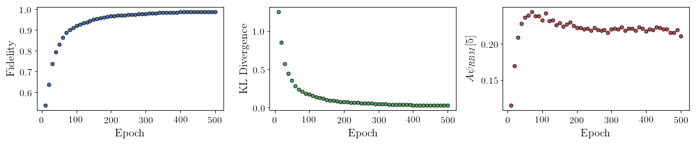
All of these training evaluators can be accessed after the training has completed, as well. The code below shows this, along with plots of each training evaluator versus the training cycle number (epoch).

[8]:

# Note that the key given to the *MetricEvaluator* must be
# what comes after callbacks[0].
fidelities = callbacks[0].Fidelity

# Alternatively, we can use the usual dictionary/list subsripting
# syntax. This is useful in cases where the name of the
# metric contains special characters or spaces.
KLs = callbacks[0]["KL"]
coeffs = callbacks[0]["A_Ψrbm_5"]

epoch = np.arange(period, epochs + 1, period)

[9]:

# Some parameters to make the plots look nice
params = {
    "text.usetex": True,
    "font.family": "serif",
    "legend.fontsize": 14,
    "figure.figsize": (10, 3),
    "axes.labelsize": 16,
    "xtick.labelsize": 14,
    "ytick.labelsize": 14,
    "lines.linewidth": 2,
    "lines.markeredgewidth": 0.8,
    "lines.markersize": 5,
    "lines.marker": "o",
    "patch.edgecolor": "black",
}
plt.rcParams.update(params)
plt.style.use("seaborn-deep")

[10]:

# Plotting
fig, axs = plt.subplots(nrows=1, ncols=3, figsize=(14, 3))
ax = axs[0]
ax.plot(epoch, fidelities, "o", color="C0", markeredgecolor="black")
ax.set_ylabel(r"Fidelity")
ax.set_xlabel(r"Epoch")

ax = axs[1]
ax.plot(epoch, KLs, "o", color="C1", markeredgecolor="black")
ax.set_ylabel(r"KL Divergence")
ax.set_xlabel(r"Epoch")

ax = axs[2]
ax.plot(epoch, coeffs, "o", color="C2", markeredgecolor="black")
ax.set_ylabel(r"$A\psi_{RBM}[5]$")
ax.set_xlabel(r"Epoch")

plt.tight_layout()
plt.savefig("fid_KL.pdf")
plt.show()

../../_images/_examples_Tutorial1_TrainPosRealWaveFunction_tutorial_quantum_ising_17_0.png

It should be noted that one could have just ran nn_state.fit(train_samples) and just used the default hyperparameters and no training evaluators.

To demonstrate how important it is to find the optimal hyperparameters for a certain system, restart this notebook and comment out the original fit statement and uncomment the one below. The default hyperparameters will be used instead. Using the non-default hyperparameters yielded a fidelity of approximately $0.994$ , while the default hyperparameters yielded a fidelity of approximately $0.523$ !

The RBM’s parameters will also be saved for future use in other tutorials. They can be saved to a pickle file with the name saved_params.pt with the code below.

[11]:

nn_state.save("saved_params.pt")

This saves the weights, visible biases and hidden biases as torch tensors with the following keys: “weights”, “visible_bias”, “hidden_bias”.