This is a static, non-editable tutorial.

We recommend you install QuCumber if you want to run the examples locally. You can then get an archive file containing the examples from the relevant release here. Alternatively, you can launch an interactive online version, though it may be a bit slow:

Reconstruction of a positive-real wavefunction¶

In this tutorial, a walkthrough of how to reconstruct a positive-real wavefunction via training a Restricted Boltzmann Machine (RBM), the neural network behind qucumber, will be presented. The data used for training will be $\sigma^{z}$ measurements from a one-dimensional transverse-field Ising model (TFIM) with 10 sites at its critical point.

Transverse-field Ising model¶

The example dataset, located in tfim1d_data.txt, comprises of 10,000 $\sigma^{z}$ measurements from a one-dimensional transverse-field Ising model (TFIM) with 10 sites at its critical point. The Hamiltonian for the transverse-field Ising model (TFIM) is given by

$\begin{equation} \mathcal{H} = -J\sum_i \sigma^z_i \sigma^z_{i+1} - h \sum_i \sigma^x_i \end{equation}$

where $\sigma^{z}_i$ is the conventional spin-1/2 Pauli operator on site $i$ . At the critical point, $J=h=1$ . As per convention, spins are represented in binary notation with zero and one denoting spin-down and spin-up, respectively.

Using qucumber to reconstruct the wavefunction¶

Imports¶

To begin the tutorial, first import the required Python packages.

[1]:

import numpy as np
import matplotlib.pyplot as plt

from qucumber.nn_states import PositiveWaveFunction
from qucumber.callbacks import MetricEvaluator

import qucumber.utils.training_statistics as ts
import qucumber.utils.data as data

The Python class PositiveWaveFunction contains generic properties of a RBM meant to reconstruct a positive-real wavefunction, the most notable one being the gradient function required for stochastic gradient descent.

To instantiate a PositiveWaveFunction object, one needs to specify the number of visible and hidden units in the RBM. The number of visible units, num_visible, is given by the size of the physical system, i.e. the number of spins or qubits (10 in this case), while the number of hidden units, num_hidden, can be varied to change the expressiveness of the neural network.

Note: The optimal num_hidden : num_visible ratio will depend on the system. For the TFIM, having this ratio be equal to 1 leads to good results with reasonable computational effort.

Training¶

To evaluate the training in real time, the fidelity between the true ground-state wavefunction of the system and the wavefunction that qucumber reconstructs, $\vert\langle\psi\vert\psi_{RBM}\rangle\vert^2$ , will be calculated along with the Kullback-Leibler (KL) divergence (the RBM’s cost function). It will also be shown that any custom function can be used to evaluate the training.

First, the training data and the true wavefunction of this system must be loaded using the data utility.

[2]:

psi_path = "tfim1d_psi.txt"
train_path = "tfim1d_data.txt"
train_data, true_psi = data.load_data(train_path, psi_path)

As previously mentioned, to instantiate a PositiveWaveFunction object, one needs to specify the number of visible and hidden units in the RBM. These two quantities equal will be kept equal.

[3]:

nv = train_data.shape[-1]
nh = nv

nn_state = PositiveWaveFunction(num_visible=nv, num_hidden=nh)
# nn_state = PositiveWaveFunction(num_visible=nv, num_hidden=nh, gpu = False)

By default, qucumber will attempt to run on a GPU if one is available (if one is not available, qucumber will default to CPU). If one wishes to run qucumber on a CPU, add the flag “gpu = False” in the PositiveWaveFunction object instantiation (i.e. uncomment the line above).

Now the hyperparameters of the training process can be specified.

epochs: the total number of training cycles that will be performed (default = 100)
pos_batch_size: the number of data points used in the positive phase of the gradient (default = 100)
neg_batch_size: the number of data points used in the negative phase of the gradient (default = pos_batch_size)
k: the number of contrastive divergence steps (default = 1)
lr: the learning rate (default = 0.001)

Note: For more information on the hyperparameters above, it is strongly encouraged that the user to read through the brief, but thorough theory document on RBMs located in the qucumber documentation. One does not have to specify these hyperparameters, as their default values will be used without the user overwriting them. It is recommended to keep with the default values until the user has a stronger grasp on what these hyperparameters mean. The quality and the computational efficiency of the training will highly depend on the choice of hyperparameters. As such, playing around with the hyperparameters is almost always necessary.

For the TFIM with 10 sites, the following hyperparameters give excellent results.

[4]:

epochs = 500
pbs = 100  # pos_batch_size
nbs = 200  # neg_batch_size
lr = 0.01
k = 10

For evaluating the training in real time, the MetricEvaluator will be called in order to calculate the training evaluators every 100 epochs. The MetricEvaluator requires the following arguments.

log_every: the frequency of the training evaluators being calculated is controlled by the log_every argument (e.g. log_every = 200 means that the MetricEvaluator will update the user every 200 epochs)
A dictionary of functions you would like to reference to evaluate the training (arguments required for these functions are keyword arguments placed after the dictionary)

The following additional arguments are needed to calculate the fidelity and KL divergence in the training_statistics utility.

target_psi: the true wavefunction of the system
space: the hilbert space of the system

The training evaluators can be printed out via the verbose=True statement.

Although the fidelity and KL divergence are excellent training evaluators, they are not practical to calculate in most cases; the user may not have access to the target wavefunction of the system, nor may generating the hilbert space of the system be computationally feasible. However, evaluating the training in real time is extremely convenient.

Any custom function that the user would like to use to evaluate the training can be given to the MetricEvaluator, thus avoiding having to calculate fidelity and/or KL divergence. Any custom function given to MetricEvaluator must take the neural-network state (in this case, the PositiveWaveFunction object) and keyword arguments. As an example, the function to be passed to the MetricEvaluator will be the fifth coefficient of the reconstructed wavefunction multiplied by a parameter, A.

[5]:

def psi_coefficient(nn_state, space, A, **kwargs):
    norm = nn_state.compute_normalization(space).sqrt_()
    return A * nn_state.psi(space)[0][4] / norm

Now the hilbert space of the system can be generated for the fidelity and KL divergence and the dictionary of functions the user would like to compute every “log_every” epochs can be given to the MetricEvaluator.

[6]:

log_every = 10
space = nn_state.generate_hilbert_space(nv)

Now the training can begin. The PositiveWaveFunction object has a property called fit which takes care of this. MetricEvaluator must be passed to the fit function in a list (callbacks).

[7]:

callbacks = [
    MetricEvaluator(
        log_every,
        {"Fidelity": ts.fidelity, "KL": ts.KL, "A_Ψrbm_5": psi_coefficient},
        target_psi=true_psi,
        verbose=True,
        space=space,
        A=3.,
    )
]

nn_state.fit(
    train_data,
    epochs=epochs,
    pos_batch_size=pbs,
    neg_batch_size=nbs,
    lr=lr,
    k=k,
    callbacks=callbacks,
)
# nn_state.fit(train_data, callbacks=callbacks)

Epoch: 10       Fidelity = 0.524441     KL = 1.311481   A_Ψrbm_5 = 0.102333
Epoch: 20       Fidelity = 0.627167     KL = 0.887134   A_Ψrbm_5 = 0.151670
Epoch: 30       Fidelity = 0.733927     KL = 0.582645   A_Ψrbm_5 = 0.194329
Epoch: 40       Fidelity = 0.794879     KL = 0.445741   A_Ψrbm_5 = 0.221883
Epoch: 50       Fidelity = 0.829248     KL = 0.363647   A_Ψrbm_5 = 0.232239
Epoch: 60       Fidelity = 0.860589     KL = 0.287518   A_Ψrbm_5 = 0.241004
Epoch: 70       Fidelity = 0.886160     KL = 0.231527   A_Ψrbm_5 = 0.244122
Epoch: 80       Fidelity = 0.902777     KL = 0.196992   A_Ψrbm_5 = 0.234641
Epoch: 90       Fidelity = 0.914448     KL = 0.174226   A_Ψrbm_5 = 0.231594
Epoch: 100      Fidelity = 0.923648     KL = 0.156510   A_Ψrbm_5 = 0.234137
Epoch: 110      Fidelity = 0.929855     KL = 0.142626   A_Ψrbm_5 = 0.220506
Epoch: 120      Fidelity = 0.937082     KL = 0.127953   A_Ψrbm_5 = 0.228048
Epoch: 130      Fidelity = 0.943320     KL = 0.114683   A_Ψrbm_5 = 0.225533
Epoch: 140      Fidelity = 0.948913     KL = 0.102805   A_Ψrbm_5 = 0.220003
Epoch: 150      Fidelity = 0.953720     KL = 0.092966   A_Ψrbm_5 = 0.219529
Epoch: 160      Fidelity = 0.957696     KL = 0.085269   A_Ψrbm_5 = 0.219721
Epoch: 170      Fidelity = 0.960716     KL = 0.079273   A_Ψrbm_5 = 0.215919
Epoch: 180      Fidelity = 0.963032     KL = 0.075418   A_Ψrbm_5 = 0.219223
Epoch: 190      Fidelity = 0.965285     KL = 0.071062   A_Ψrbm_5 = 0.217072
Epoch: 200      Fidelity = 0.966294     KL = 0.069517   A_Ψrbm_5 = 0.218791
Epoch: 210      Fidelity = 0.968279     KL = 0.065436   A_Ψrbm_5 = 0.214237
Epoch: 220      Fidelity = 0.969002     KL = 0.063958   A_Ψrbm_5 = 0.208316
Epoch: 230      Fidelity = 0.970735     KL = 0.060499   A_Ψrbm_5 = 0.211827
Epoch: 240      Fidelity = 0.971954     KL = 0.058173   A_Ψrbm_5 = 0.213458
Epoch: 250      Fidelity = 0.972797     KL = 0.056356   A_Ψrbm_5 = 0.216414
Epoch: 260      Fidelity = 0.973940     KL = 0.054098   A_Ψrbm_5 = 0.219072
Epoch: 270      Fidelity = 0.975173     KL = 0.051311   A_Ψrbm_5 = 0.213439
Epoch: 280      Fidelity = 0.976146     KL = 0.049353   A_Ψrbm_5 = 0.214791
Epoch: 290      Fidelity = 0.977626     KL = 0.046184   A_Ψrbm_5 = 0.215294
Epoch: 300      Fidelity = 0.978880     KL = 0.043539   A_Ψrbm_5 = 0.215247
Epoch: 310      Fidelity = 0.979931     KL = 0.041293   A_Ψrbm_5 = 0.211467
Epoch: 320      Fidelity = 0.981140     KL = 0.038849   A_Ψrbm_5 = 0.213601
Epoch: 330      Fidelity = 0.982012     KL = 0.036976   A_Ψrbm_5 = 0.216033
Epoch: 340      Fidelity = 0.982764     KL = 0.035460   A_Ψrbm_5 = 0.217036
Epoch: 350      Fidelity = 0.983499     KL = 0.033983   A_Ψrbm_5 = 0.208566
Epoch: 360      Fidelity = 0.984789     KL = 0.031407   A_Ψrbm_5 = 0.218186
Epoch: 370      Fidelity = 0.985142     KL = 0.030643   A_Ψrbm_5 = 0.215245
Epoch: 380      Fidelity = 0.985985     KL = 0.028931   A_Ψrbm_5 = 0.217562
Epoch: 390      Fidelity = 0.986345     KL = 0.028262   A_Ψrbm_5 = 0.217989
Epoch: 400      Fidelity = 0.986798     KL = 0.027449   A_Ψrbm_5 = 0.215068
Epoch: 410      Fidelity = 0.987459     KL = 0.026076   A_Ψrbm_5 = 0.220650
Epoch: 420      Fidelity = 0.987785     KL = 0.025427   A_Ψrbm_5 = 0.220902
Epoch: 430      Fidelity = 0.988085     KL = 0.024916   A_Ψrbm_5 = 0.217657
Epoch: 440      Fidelity = 0.988270     KL = 0.024565   A_Ψrbm_5 = 0.218701
Epoch: 450      Fidelity = 0.988164     KL = 0.024811   A_Ψrbm_5 = 0.222711
Epoch: 460      Fidelity = 0.988564     KL = 0.024018   A_Ψrbm_5 = 0.212042
Epoch: 470      Fidelity = 0.988859     KL = 0.023432   A_Ψrbm_5 = 0.221610
Epoch: 480      Fidelity = 0.989148     KL = 0.022804   A_Ψrbm_5 = 0.224286
Epoch: 490      Fidelity = 0.989477     KL = 0.022194   A_Ψrbm_5 = 0.223508
Epoch: 500      Fidelity = 0.989738     KL = 0.021626   A_Ψrbm_5 = 0.223838

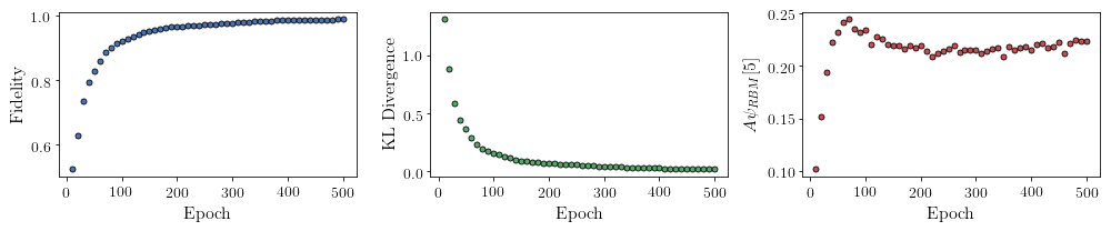
All of these training evaluators can be accessed after the training has completed, as well. The code below shows this, along with plots of each training evaluator versus the training cycle number (epoch).

[8]:

fidelities = callbacks[0].Fidelity
KLs = callbacks[0].KL
coeffs = callbacks[0].A_Ψrbm_5
# Please note that the key given to the *MetricEvaluator* must be what comes after callbacks[0].
epoch = np.arange(log_every, epochs + 1, log_every)

[9]:

# Some parameters to make the plots look nice
params = {'text.usetex': True,
            'font.family': 'serif',
            'legend.fontsize': 14,
            'figure.figsize': (10, 3),
            'axes.labelsize': 16,
            'xtick.labelsize':14,
            'ytick.labelsize':14,
            'lines.linewidth':2,
            'lines.markeredgewidth': 0.8,
            'lines.markersize': 5,
            'lines.marker': "o",
            "patch.edgecolor": "black"
         }
plt.rcParams.update(params)
plt.style.use('seaborn-deep')

[10]:

# Plotting
fig, axs = plt.subplots(nrows=1, ncols=3, figsize=(14, 3))
ax = axs[0]
ax.plot(epoch, fidelities, "o", color = "C0", markeredgecolor="black")
ax.set_ylabel(r'Fidelity')
ax.set_xlabel(r'Epoch')

ax = axs[1]
ax.plot(epoch, KLs, "o", color = "C1", markeredgecolor="black")
ax.set_ylabel(r'KL Divergence')
ax.set_xlabel(r'Epoch')

ax = axs[2]
ax.plot(epoch, coeffs, "o", color = "C2", markeredgecolor="black")
ax.set_ylabel(r'$A\psi_{RBM}[5]$')
ax.set_xlabel(r'Epoch')

plt.tight_layout()
plt.savefig("fid_KL.pdf")
plt.show()

../../_images/_examples_Tutorial1_TrainPosRealWaveFunction_tutorial_quantum_ising_17_0.png

It should be noted that one could have just ran nn_state.fit(train_samples) and just used the default hyperparameters and no training evaluators.

To demonstrate how important it is to find the optimal hyperparameters for a certain system, restart this notebook and comment out the original fit statement and uncomment the one below. The default hyperparameters will be used instead. Using the non-default hyperparameters yielded a fidelity of approximately 0.994, while the default hyperparameters yielded a fidelity of approximately 0.523!

The RBM’s parameters will also be saved for future use in other tutorials. They can be saved to a pickle file with the name “saved_params.pt” with the code below.

[11]:

nn_state.save("saved_params.pt")

This saves the weights, visible biases and hidden biases as torch tensors with the following keys: “weights”, “visible_bias”, “hidden_bias”.