This is a static, non-editable tutorial.

We recommend you install QuCumber if you want to run the examples locally. You can then get an archive file containing the examples from the relevant release here. Alternatively, you can launch an interactive online version, though it may be a bit slow:

Reconstruction of a complex wavefunction¶

In this tutorial, a walkthrough of how to reconstruct a complex wavefunction via training a Restricted Boltzmann Machine (RBM), the neural network behind qucumber, will be presented.

The wavefunction to be reconstructed¶

The simple wavefunction below describing two qubits (coefficients stored in qubits_psi.txt) will be reconstructed.

$\begin{equation} \vert\psi \rangle = \alpha \vert00\rangle + \beta \vert 01\rangle + \gamma \vert10\rangle + \delta \vert11\rangle \end{equation}$

where the exact values of $\alpha, \beta, \gamma$ and $\delta$ used for this tutorial are

$\begin{align} \alpha & = 0.2861 + 0.0539 i \\ \beta & = 0.3687 - 0.3023 i \\ \gamma & = -0.1672 - 0.3529 i \\ \delta & = -0.5659 - 0.4639 i. \end{align}$

The example dataset, qubits_train.txt, comprises of 500 $\sigma$ measurements made in various bases (X, Y and Z). A corresponding file containing the bases for each data point in qubits_train.txt, qubits_train_bases.txt, is also required. As per convention, spins are represented in binary notation with zero and one denoting spin-down and spin-up, respectively.

Using qucumber to reconstruct the wavefunction¶

Imports¶

To begin the tutorial, first import the required Python packages.

[1]:

import numpy as np
import torch
import matplotlib.pyplot as plt

from qucumber.nn_states import ComplexWaveFunction

from qucumber.callbacks import MetricEvaluator

import qucumber.utils.unitaries as unitaries
import qucumber.utils.cplx as cplx

import qucumber.utils.training_statistics as ts
import qucumber.utils.data as data

The Python class ComplexWaveFunction contains generic properties of a RBM meant to reconstruct a complex wavefunction, the most notable one being the gradient function required for stochastic gradient descent.

To instantiate a ComplexWaveFunction object, one needs to specify the number of visible and hidden units in the RBM. The number of visible units, num_visible, is given by the size of the physical system, i.e. the number of spins or qubits (2 in this case), while the number of hidden units, num_hidden, can be varied to change the expressiveness of the neural network.

Note: The optimal num_hidden : num_visible ratio will depend on the system. For the two-qubit wavefunction described above, good results are yielded when this ratio is 1.

On top of needing the number of visible and hidden units, a ComplexWaveFunction object requires the user to input a dictionary containing the unitary operators (2x2) that will be used to rotate the qubits in and out of the computational basis, Z, during the training process. The unitaries utility will take care of creating this dictionary.

The MetricEvaluator class and training_statistics utility are built-in amenities that will allow the user to evaluate the training in real time.

Lastly, the cplx utility allows qucumber to be able to handle complex numbers. Currently, Pytorch does not support complex numbers.

Training¶

To evaluate the training in real time, the fidelity between the true wavefunction of the system and the wavefunction that qucumber reconstructs, $\vert\langle\psi\vert\psi_{RBM}\rangle\vert^2$ , will be calculated along with the Kullback-Leibler (KL) divergence (the RBM’s cost function). First, the training data and the true wavefunction of this system need to be loaded using the data utility.

[2]:

train_path = "qubits_train.txt"
train_bases_path = "qubits_train_bases.txt"
psi_path = "qubits_psi.txt"
bases_path = "qubits_bases.txt"

train_samples, true_psi, train_bases, bases = data.load_data(
    train_path, psi_path, train_bases_path, bases_path
)

The file qubits_bases.txt contains every unique basis in the qubits_train_bases.txt file. Calculation of the full KL divergence in every basis requires the user to specify each unique basis.

As previouosly mentioned, a ComplexWaveFunction object requires a dictionary that contains the unitariy operators that will be used to rotate the qubits in and out of the computational basis, Z, during the training process. In the case of the provided dataset, the unitaries required are the well-known $H$ , and $K$ gates. The dictionary needed can be created with the following command.

[3]:

unitary_dict = unitaries.create_dict()
# unitary_dict = unitaries.create_dict(unitary_name=torch.tensor([[real part],
#                                                                 [imaginary part]],
#                                                                 dtype=torch.double)

If the user wishes to add their own unitary operators from their experiment to unitary_dict, uncomment the block above. When unitaries.create_dict() is called, it will contain the identity and the $H$ and $K$ gates by default with the keys “Z”, “X” and “Y”, respectively.

The number of visible units in the RBM is equal to the number of qubits. The number of hidden units will also be taken to be the number of visible units.

[4]:

nv = train_samples.shape[-1]
nh = nv

nn_state = ComplexWaveFunction(
    num_visible=nv, num_hidden=nh, unitary_dict=unitary_dict, gpu=False
)
# nn_state = ComplexWaveFunction(num_visible=nv, num_hidden=nh, unitary_dict=unitary_dict)

By default, qucumber will attempt to run on a GPU if one is available (if one is not available, qucumber will default to CPU). If one wishes to run qucumber on a CPU, add the flag “gpu = False” in the ComplexWaveFunction object instantiation. Uncomment the line above to run this tutorial on a GPU.

Now the hyperparameters of the training process can be specified.

epochs: the total number of training cycles that will be performed (default = 100)
pos_batch_size: the number of data points used in the positive phase of the gradient (default = 100)
neg_batch_size: the number of data points used in the negative phase of the gradient (default = pos_batch_size)
k: the number of contrastive divergence steps (default = 1)
lr: the learning rate (default = 0.001)

Note: For more information on the hyperparameters above, it is strongly encouraged that the user to read through the brief, but thorough theory document on RBMs. One does not have to specify these hyperparameters, as their default values will be used without the user overwriting them. It is recommended to keep with the default values until the user has a stronger grasp on what these hyperparameters mean. The quality and the computational efficiency of the training will highly depend on the choice of hyperparameters. As such, playing around with the hyperparameters is almost always necessary.

The two-qubit example in this tutorial should be extremely easy to train, regardless of the choice of hyperparameters. However, the hyperparameters below will be used.

[5]:

epochs = 100
pbs = 50  # pos_batch_size
nbs = 50  # neg_batch_size
lr = 0.1
k = 5

For evaluating the training in real time, the MetricEvaluator will be called to calculate the training evaluators every 10 epochs. The MetricEvaluator requires the following arguments.

log_every: the frequency of the training evaluators being calculated is controlled by the log_every argument (e.g. log_every = 200 means that the MetricEvaluator will update the user every 200 epochs)
A dictionary of functions you would like to reference to evaluate the training (arguments required for these functions are keyword arguments placed after the dictionary)

The following additional arguments are needed to calculate the fidelity and KL divergence in the training_statistics utility.

target_psi (the true wavefunction of the system)
space (the hilbert space of the system)

The training evaluators can be printed out via the verbose=True statement.

Although the fidelity and KL divergence are excellent training evaluators, they are not practical to calculate in most cases; the user may not have access to the target wavefunction of the system, nor may generating the hilbert space of the system be computationally feasible. However, evaluating the training in real time is extremely convenient.

Any custom function that the user would like to use to evaluate the training can be given to the MetricEvaluator, thus avoiding having to calculate fidelity and/or KL divergence. As an example, functions that calculate the the norm of each of the reconstructed wavefunction’s coefficients are presented. Any custom function given to MetricEvaluator must take the neural-network state (in this case, the ComplexWaveFunction object) and keyword arguments. Although the given example requires the hilbert space to be computed, the scope of the MetricEvaluator’s ability to be able to handle any function should still be evident.

[6]:

def alpha(nn_state, space, **kwargs):
    rbm_psi = nn_state.psi(space)
    normalization = nn_state.compute_normalization(space).sqrt_()
    alpha_ = cplx.norm(
        torch.tensor([rbm_psi[0][0], rbm_psi[1][0]], device=nn_state.device)
        / normalization
    )

    return alpha_


def beta(nn_state, space, **kwargs):
    rbm_psi = nn_state.psi(space)
    normalization = nn_state.compute_normalization(space).sqrt_()
    beta_ = cplx.norm(
        torch.tensor([rbm_psi[0][1], rbm_psi[1][1]], device=nn_state.device)
        / normalization
    )

    return beta_


def gamma(nn_state, space, **kwargs):
    rbm_psi = nn_state.psi(space)
    normalization = nn_state.compute_normalization(space).sqrt_()
    gamma_ = cplx.norm(
        torch.tensor([rbm_psi[0][2], rbm_psi[1][2]], device=nn_state.device)
        / normalization
    )

    return gamma_


def delta(nn_state, space, **kwargs):
    rbm_psi = nn_state.psi(space)
    normalization = nn_state.compute_normalization(space).sqrt_()
    delta_ = cplx.norm(
        torch.tensor([rbm_psi[0][3], rbm_psi[1][3]], device=nn_state.device)
        / normalization
    )

    return delta_

Now the hilbert space of the system must be generated for the fidelity and KL divergence and the dictionary of functions the user would like to compute every “log_every” epochs must be given to the MetricEvaluator.

[7]:

log_every = 2
space = nn_state.generate_hilbert_space(nv)

callbacks = [
    MetricEvaluator(
        log_every,
        {
            "Fidelity": ts.fidelity,
            "KL": ts.KL,
            "normα": alpha,
#             "normβ": beta,
#             "normγ": gamma,
#             "normδ": delta,
        },
        target_psi=true_psi,
        bases=bases,
        verbose=True,
        space=space,
    )
]

Now the training can begin. The ComplexWaveFunction object has a property called fit which takes care of this.

[8]:

nn_state.fit(
    train_samples,
    epochs=epochs,
    pos_batch_size=pbs,
    neg_batch_size=nbs,
    lr=lr,
    k=k,
    input_bases=train_bases,
    callbacks=callbacks,
)

Epoch: 2        Fidelity = 0.609290     KL = 0.251365   normα = 0.328561
Epoch: 4        Fidelity = 0.761520     KL = 0.130756   normα = 0.268571
Epoch: 6        Fidelity = 0.838254     KL = 0.082158   normα = 0.253614
Epoch: 8        Fidelity = 0.882321     KL = 0.059876   normα = 0.251210
Epoch: 10       Fidelity = 0.909942     KL = 0.046754   normα = 0.259010
Epoch: 12       Fidelity = 0.929755     KL = 0.036943   normα = 0.258238
Epoch: 14       Fidelity = 0.942398     KL = 0.030965   normα = 0.262524
Epoch: 16       Fidelity = 0.951771     KL = 0.027162   normα = 0.250808
Epoch: 18       Fidelity = 0.958536     KL = 0.023913   normα = 0.257332
Epoch: 20       Fidelity = 0.963766     KL = 0.021570   normα = 0.259561
Epoch: 22       Fidelity = 0.968224     KL = 0.019610   normα = 0.263528
Epoch: 24       Fidelity = 0.970991     KL = 0.018523   normα = 0.256601
Epoch: 26       Fidelity = 0.974414     KL = 0.017127   normα = 0.256168
Epoch: 28       Fidelity = 0.976543     KL = 0.016030   normα = 0.261707
Epoch: 30       Fidelity = 0.977891     KL = 0.015551   normα = 0.254371
Epoch: 32       Fidelity = 0.978768     KL = 0.015847   normα = 0.242762
Epoch: 34       Fidelity = 0.981126     KL = 0.013974   normα = 0.259100
Epoch: 36       Fidelity = 0.981330     KL = 0.013704   normα = 0.262152
Epoch: 38       Fidelity = 0.981989     KL = 0.013495   normα = 0.256111
Epoch: 40       Fidelity = 0.983230     KL = 0.012711   normα = 0.269000
Epoch: 42       Fidelity = 0.984230     KL = 0.012301   normα = 0.273091
Epoch: 44       Fidelity = 0.984190     KL = 0.012178   normα = 0.260481
Epoch: 46       Fidelity = 0.985494     KL = 0.011501   normα = 0.269168
Epoch: 48       Fidelity = 0.985192     KL = 0.011518   normα = 0.269217
Epoch: 50       Fidelity = 0.986754     KL = 0.010896   normα = 0.264035
Epoch: 52       Fidelity = 0.987266     KL = 0.011288   normα = 0.263792
Epoch: 54       Fidelity = 0.987998     KL = 0.010323   normα = 0.268859
Epoch: 56       Fidelity = 0.987993     KL = 0.009957   normα = 0.267215
Epoch: 58       Fidelity = 0.988191     KL = 0.009873   normα = 0.273412
Epoch: 60       Fidelity = 0.988129     KL = 0.009665   normα = 0.264751
Epoch: 62       Fidelity = 0.986891     KL = 0.010557   normα = 0.254349
Epoch: 64       Fidelity = 0.988134     KL = 0.009504   normα = 0.264387
Epoch: 66       Fidelity = 0.987419     KL = 0.009870   normα = 0.263105
Epoch: 68       Fidelity = 0.988299     KL = 0.009280   normα = 0.264269
Epoch: 70       Fidelity = 0.989128     KL = 0.008897   normα = 0.267263
Epoch: 72       Fidelity = 0.989572     KL = 0.008808   normα = 0.268239
Epoch: 74       Fidelity = 0.988996     KL = 0.008901   normα = 0.256966
Epoch: 76       Fidelity = 0.988131     KL = 0.009278   normα = 0.261540
Epoch: 78       Fidelity = 0.989458     KL = 0.008405   normα = 0.263894
Epoch: 80       Fidelity = 0.988967     KL = 0.008628   normα = 0.261319
Epoch: 82       Fidelity = 0.989337     KL = 0.008332   normα = 0.271008
Epoch: 84       Fidelity = 0.989170     KL = 0.008351   normα = 0.270172
Epoch: 86       Fidelity = 0.989256     KL = 0.008291   normα = 0.273329
Epoch: 88       Fidelity = 0.989592     KL = 0.008019   normα = 0.269137
Epoch: 90       Fidelity = 0.989677     KL = 0.007917   normα = 0.266120
Epoch: 92       Fidelity = 0.989260     KL = 0.008174   normα = 0.261290
Epoch: 94       Fidelity = 0.990006     KL = 0.007627   normα = 0.266389
Epoch: 96       Fidelity = 0.989957     KL = 0.007610   normα = 0.270035
Epoch: 98       Fidelity = 0.990623     KL = 0.007506   normα = 0.278505
Epoch: 100      Fidelity = 0.990754     KL = 0.007096   normα = 0.266719

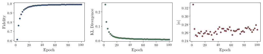
All of these training evaluators can be accessed after the training has completed, as well. The code below shows this, along with plots of each training evaluator versus the training cycle number (epoch).

[9]:

fidelities = callbacks[0].Fidelity
KLs = callbacks[0].KL
coeffs = callbacks[0].normα
# Please note that the key given to the *MetricEvaluator* must be what comes after callbacks[0].
epoch = np.arange(log_every, epochs + 1, log_every)

[10]:

# Some parameters to make the plots look nice
params = {'text.usetex': True,
            'font.family': 'serif',
            'legend.fontsize': 14,
            'figure.figsize': (10, 3),
            'axes.labelsize': 16,
            'xtick.labelsize':14,
            'ytick.labelsize':14,
            'lines.linewidth':2,
            'lines.markeredgewidth': 0.8,
            'lines.markersize': 5,
            'lines.marker': "o",
            "patch.edgecolor": "black"
         }
plt.rcParams.update(params)
plt.style.use('seaborn-deep')

[11]:

fig, axs = plt.subplots(nrows=1, ncols=3, figsize=(14, 3))
ax = axs[0]
ax.plot(epoch, fidelities, "o", color = "C0", markeredgecolor="black")
ax.set_ylabel(r'Fidelity')
ax.set_xlabel(r'Epoch')

ax = axs[1]
ax.plot(epoch, KLs, "o", color = "C1", markeredgecolor="black")
ax.set_ylabel(r'KL Divergence')
ax.set_xlabel(r'Epoch')

ax = axs[2]
ax.plot(epoch, coeffs, "o", color = "C2", markeredgecolor="black")
ax.set_ylabel(r'$\vert\alpha\vert$')
ax.set_xlabel(r'Epoch')

plt.tight_layout()
plt.savefig("complex_fid_KL.pdf")
plt.show()

../../_images/_examples_Tutorial2_TrainComplexWaveFunction_tutorial_qubits_19_0.png

It should be noted that one could have just ran nn_state.fit(train_samples) and just used the default hyperparameters and no training evaluators.

At the end of the training process, the network parameters (the weights, visible biases and hidden biases) are stored in the ComplexWaveFunction object. One can save them to a pickle file, which will be called saved_params.pt, with the following command.

[12]:

nn_state.save("saved_params.pt")

This saves the weights, visible biases and hidden biases as torch tensors with the following keys: “weights”, “visible_bias”, “hidden_bias”.