This is a static, non-editable tutorial.

We recommend you install QuCumber if you want to run the examples locally. You can then get an archive file containing the examples from the relevant release here. Alternatively, you can launch an interactive online version, though it may be a bit slow:

Reconstruction of a positive-real wavefunction

This tutorial shows how to reconstruct a positive-real wavefunction via training a Restricted Boltzmann Machine (RBM), the neural network behind QuCumber. The data used for training are measurements from a one-dimensional transverse-field Ising model (TFIM) with 10 sites at its critical point.

Transverse-field Ising model

The example dataset, located in tfim1d_data.txt, comprises 10,000 measurements from a one-dimensional TFIM with 10 sites at its critical point. The Hamiltonian for the TFIM is given by

where is the conventional spin-1/2 Pauli operator on site . At the critical point, . By convention, spins are represented in binary notation with zero and one denoting the states spin-down and spin-up, respectively.

Using QuCumber to reconstruct the wavefunction

Imports

To begin the tutorial, first import the required Python packages.

import numpy as np
import matplotlib.pyplot as plt

from qucumber.nn_states import PositiveWaveFunction
from qucumber.callbacks import MetricEvaluator

import qucumber.utils.training_statistics as ts
import qucumber.utils.data as data
import qucumber

# set random seed on cpu but not gpu, since we won't use gpu for this tutorial
qucumber.set_random_seed(1234, cpu=True, gpu=False)

The Python class PositiveWaveFunction contains generic properties of a RBM meant to reconstruct a positive-real wavefunction, the most notable one being the gradient function required for stochastic gradient descent.

To instantiate a PositiveWaveFunction object, one needs to specify the number of visible and hidden units in the RBM. The number of visible units, num_visible, is given by the size of the physical system, i.e. the number of spins or qubits (10 in this case), while the number of hidden units, num_hidden, can be varied to change the expressiveness of the neural network.

Note: The optimal num_hidden : num_visible ratio will depend on the system. For the TFIM, having this ratio be equal to 1 leads to good results with reasonable computational effort.

Training

To evaluate the training in real time, we compute the fidelity between the true ground-state wavefunction of the system and the wavefunction that QuCumber reconstructs, , along with the Kullback-Leibler (KL) divergence (the RBM’s cost function). As will be shown below, any custom function can be used to evaluate the training.

First, the training data and the true wavefunction of this system must be loaded using the data utility.

psi_path = "tfim1d_psi.txt"
train_path = "tfim1d_data.txt"
train_data, true_psi = data.load_data(train_path, psi_path)

As previously mentioned, to instantiate a PositiveWaveFunction object, one needs to specify the number of visible and hidden units in the RBM; we choose them to be equal.

nv = train_data.shape[-1]
nh = nv

nn_state = PositiveWaveFunction(num_visible=nv, num_hidden=nh, gpu=False)

If gpu=True (the default), QuCumber will attempt to run on a GPU if one is available (otherwise, QuCumber will default to CPU). If one gpu=False, QuCumber will run on the CPU.

Now we specify the hyperparameters of the training process:

1. epochs: the total number of training cycles that will be performed (default = 100)

2. pbs (pos_batch_size): the number of data points used in the positive phase of the gradient (default = 100)

3. nbs (neg_batch_size): the number of data points used in the negative phase of the gradient (default = 100)

4. k: the number of contrastive divergence steps (default = 1)

5. lr: the learning rate (default = 0.001)

   Note: For more information on the hyperparameters above, it is strongly encouraged that the user to read through the brief, but thorough theory document on RBMs located in the QuCumber documentation. One does not have to specify these hyperparameters, as their default values will be used without the user overwriting them. It is recommended to keep with the default values until the user has a stronger grasp on what these hyperparameters mean. The quality and the computational efficiency of the training will highly depend on the choice of hyperparameters. As such, playing around with the hyperparameters is almost always necessary.

For the TFIM with 10 sites, the following hyperparameters give excellent results:

epochs = 500
pbs = 100
nbs = pbs
lr = 0.01
k = 10

For evaluating the training in real time, the MetricEvaluator is called every 100 epochs in order to calculate the training evaluators. The MetricEvaluator requires the following arguments:

1. period: the frequency of the training evaluators being calculated (e.g. period=100 means that the MetricEvaluator will do an evaluation every 100 epochs)

2. A dictionary of functions you would like to reference to evaluate the training (arguments required for these functions are keyword arguments placed after the dictionary)

The following additional arguments are needed to calculate the fidelity and KL divergence in the training_statistics utility:

• target_psi: the true wavefunction of the system

• space: the Hilbert space of the system

The training evaluators can be printed out via the verbose=True statement.

Although the fidelity and KL divergence are excellent training evaluators, they are not practical to calculate in most cases; the user may not have access to the target wavefunction of the system, nor may generating the Hilbert space of the system be computationally feasible. However, evaluating the training in real time is extremely convenient.

Any custom function that the user would like to use to evaluate the training can be given to the MetricEvaluator, thus avoiding having to calculate fidelity and/or KL divergence. Any custom function given to MetricEvaluator must take the neural-network state (in this case, the PositiveWaveFunction object) and keyword arguments. As an example, we define a custom function psi_coefficient, which is the fifth coefficient of the reconstructed wavefunction multiplied by a parameter .

def psi_coefficient(nn_state, space, A, **kwargs):
    norm = nn_state.compute_normalization(space).sqrt_()
    return A * nn_state.psi(space)[0][4] / norm

Now the Hilbert space of the system can be generated for the fidelity and KL divergence.

period = 10
space = nn_state.generate_hilbert_space()

Now the training can begin. The PositiveWaveFunction object has a property called fit which takes care of this. MetricEvaluator must be passed to the fit function in a list (callbacks).

callbacks = [
    MetricEvaluator(
        period,
        {"Fidelity": ts.fidelity, "KL": ts.KL, "A_Ψrbm_5": psi_coefficient},
        target=true_psi,
        verbose=True,
        space=space,
        A=3.0,
    )
]

nn_state.fit(
    train_data,
    epochs=epochs,
    pos_batch_size=pbs,
    neg_batch_size=nbs,
    lr=lr,
    k=k,
    callbacks=callbacks,
    time=True,
)

Epoch: 10       Fidelity = 0.500444     KL = 1.434037   A_Ψrbm_5 = 0.111008
Epoch: 20       Fidelity = 0.570243     KL = 1.098804   A_Ψrbm_5 = 0.140842
Epoch: 30       Fidelity = 0.681689     KL = 0.712384   A_Ψrbm_5 = 0.192823
Epoch: 40       Fidelity = 0.781095     KL = 0.457683   A_Ψrbm_5 = 0.222722
Epoch: 50       Fidelity = 0.840074     KL = 0.326949   A_Ψrbm_5 = 0.239039
Epoch: 60       Fidelity = 0.875057     KL = 0.252105   A_Ψrbm_5 = 0.239344
Epoch: 70       Fidelity = 0.895826     KL = 0.211282   A_Ψrbm_5 = 0.239159
Epoch: 80       Fidelity = 0.907819     KL = 0.190410   A_Ψrbm_5 = 0.245369
Epoch: 90       Fidelity = 0.914834     KL = 0.177129   A_Ψrbm_5 = 0.238663
Epoch: 100      Fidelity = 0.920255     KL = 0.167432   A_Ψrbm_5 = 0.246280
Epoch: 110      Fidelity = 0.924585     KL = 0.158587   A_Ψrbm_5 = 0.244731
Epoch: 120      Fidelity = 0.928158     KL = 0.150159   A_Ψrbm_5 = 0.236318
Epoch: 130      Fidelity = 0.932489     KL = 0.140405   A_Ψrbm_5 = 0.243707
Epoch: 140      Fidelity = 0.936930     KL = 0.130399   A_Ψrbm_5 = 0.242923
Epoch: 150      Fidelity = 0.941502     KL = 0.120001   A_Ψrbm_5 = 0.246340
Epoch: 160      Fidelity = 0.946511     KL = 0.108959   A_Ψrbm_5 = 0.243519
Epoch: 170      Fidelity = 0.951172     KL = 0.098144   A_Ψrbm_5 = 0.235464
Epoch: 180      Fidelity = 0.955645     KL = 0.088780   A_Ψrbm_5 = 0.237005
Epoch: 190      Fidelity = 0.959723     KL = 0.080219   A_Ψrbm_5 = 0.234366
Epoch: 200      Fidelity = 0.962512     KL = 0.074663   A_Ψrbm_5 = 0.227764
Epoch: 210      Fidelity = 0.965615     KL = 0.068804   A_Ψrbm_5 = 0.233611
Epoch: 220      Fidelity = 0.967394     KL = 0.065302   A_Ψrbm_5 = 0.233936
Epoch: 230      Fidelity = 0.969286     KL = 0.061641   A_Ψrbm_5 = 0.230911
Epoch: 240      Fidelity = 0.970506     KL = 0.059283   A_Ψrbm_5 = 0.225389
Epoch: 250      Fidelity = 0.971461     KL = 0.057742   A_Ψrbm_5 = 0.233186
Epoch: 260      Fidelity = 0.973525     KL = 0.053430   A_Ψrbm_5 = 0.225180
Epoch: 270      Fidelity = 0.975005     KL = 0.050646   A_Ψrbm_5 = 0.228983
Epoch: 280      Fidelity = 0.976041     KL = 0.048451   A_Ψrbm_5 = 0.231805
Epoch: 290      Fidelity = 0.977197     KL = 0.046058   A_Ψrbm_5 = 0.232667
Epoch: 300      Fidelity = 0.977386     KL = 0.045652   A_Ψrbm_5 = 0.239462
Epoch: 310      Fidelity = 0.979153     KL = 0.042036   A_Ψrbm_5 = 0.232371
Epoch: 320      Fidelity = 0.979264     KL = 0.041764   A_Ψrbm_5 = 0.224176
Epoch: 330      Fidelity = 0.981203     KL = 0.037786   A_Ψrbm_5 = 0.231017
Epoch: 340      Fidelity = 0.982122     KL = 0.035848   A_Ψrbm_5 = 0.233144
Epoch: 350      Fidelity = 0.982408     KL = 0.035287   A_Ψrbm_5 = 0.239080
Epoch: 360      Fidelity = 0.983737     KL = 0.032537   A_Ψrbm_5 = 0.232325
Epoch: 370      Fidelity = 0.984651     KL = 0.030705   A_Ψrbm_5 = 0.233523
Epoch: 380      Fidelity = 0.985230     KL = 0.029546   A_Ψrbm_5 = 0.235031
Epoch: 390      Fidelity = 0.985815     KL = 0.028345   A_Ψrbm_5 = 0.235860
Epoch: 400      Fidelity = 0.986262     KL = 0.027459   A_Ψrbm_5 = 0.240407
Epoch: 410      Fidelity = 0.986678     KL = 0.026623   A_Ψrbm_5 = 0.229870
Epoch: 420      Fidelity = 0.987422     KL = 0.025197   A_Ψrbm_5 = 0.235147
Epoch: 430      Fidelity = 0.987339     KL = 0.025400   A_Ψrbm_5 = 0.227832
Epoch: 440      Fidelity = 0.988037     KL = 0.023930   A_Ψrbm_5 = 0.237405
Epoch: 450      Fidelity = 0.988104     KL = 0.023838   A_Ψrbm_5 = 0.241163
Epoch: 460      Fidelity = 0.988751     KL = 0.022605   A_Ψrbm_5 = 0.233818
Epoch: 470      Fidelity = 0.988836     KL = 0.022364   A_Ψrbm_5 = 0.241944
Epoch: 480      Fidelity = 0.989127     KL = 0.021844   A_Ψrbm_5 = 0.235669
Epoch: 490      Fidelity = 0.989361     KL = 0.021288   A_Ψrbm_5 = 0.242225
Epoch: 500      Fidelity = 0.989816     KL = 0.020486   A_Ψrbm_5 = 0.232313
Total time elapsed during training: 87.096 s

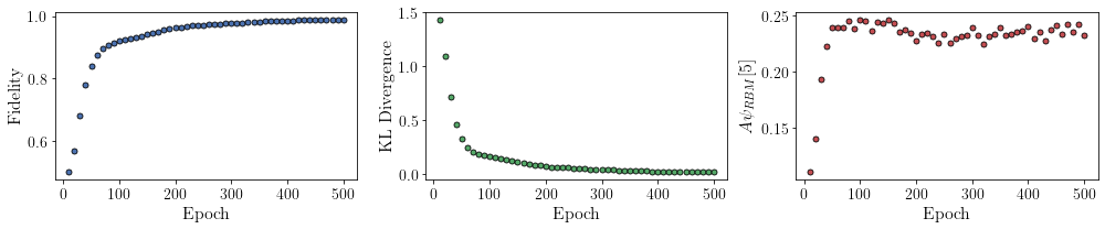
All of these training evaluators can be accessed after the training has completed. The code below shows this, along with plots of each training evaluator as a function of epoch (training cycle number).

# Note that the key given to the *MetricEvaluator* must be
# what comes after callbacks[0].
fidelities = callbacks[0].Fidelity

# Alternatively, we can use the usual dictionary/list subsripting
# syntax. This is useful in cases where the name of the
# metric contains special characters or spaces.
KLs = callbacks[0]["KL"]
coeffs = callbacks[0]["A_Ψrbm_5"]

epoch = np.arange(period, epochs + 1, period)

# Some parameters to make the plots look nice
params = {
    "text.usetex": True,
    "font.family": "serif",
    "legend.fontsize": 14,
    "figure.figsize": (10, 3),
    "axes.labelsize": 16,
    "xtick.labelsize": 14,
    "ytick.labelsize": 14,
    "lines.linewidth": 2,
    "lines.markeredgewidth": 0.8,
    "lines.markersize": 5,
    "lines.marker": "o",
    "patch.edgecolor": "black",
}
plt.rcParams.update(params)
plt.style.use("seaborn-deep")

# Plotting
fig, axs = plt.subplots(nrows=1, ncols=3, figsize=(14, 3))
ax = axs[0]
ax.plot(epoch, fidelities, "o", color="C0", markeredgecolor="black")
ax.set_ylabel(r"Fidelity")
ax.set_xlabel(r"Epoch")

ax = axs[1]
ax.plot(epoch, KLs, "o", color="C1", markeredgecolor="black")
ax.set_ylabel(r"KL Divergence")
ax.set_xlabel(r"Epoch")

ax = axs[2]
ax.plot(epoch, coeffs, "o", color="C2", markeredgecolor="black")
ax.set_ylabel(r"$A\psi_{RBM}[5]$")
ax.set_xlabel(r"Epoch")

plt.tight_layout()
plt.show()

It should be noted that one could have just ran nn_state.fit(train_samples), which uses the default hyperparameters and no training evaluators.

To demonstrate how important it is to find the optimal hyperparameters for a certain system, restart this notebook and comment out the original fit statement, then uncomment and run the cell below.

# nn_state.fit(train_samples)

Using the non-default hyperparameters produced a fidelity of approximately , while the default hyperparameters yield approximately !

The trained RBM can be saved to a pickle file with the name saved_params.pt for future use:

nn_state.save("saved_params.pt")

This saves the weights, visible biases and hidden biases as torch tensors under the following keys: weights, visible_bias, hidden_bias.